Introduction to `pandas`

The pandas library (https://pandas.pydata.org) is one of the most used tool at the disposal of people working with data in python today.

It allows to crunch data easily
It mainly provides a DataFrame object (a table of data) with a huge set of functionalities

Why ?

Through pandas, you get acquainted with your data by analyzing it

What’s the average, median, max, or min of each column?
Does column A correlate with column B?
What does the distribution of data in column C look like?

Why (con’t) ?

you get acquainted with your data by cleaning and transforming it

Removing missing values, filter rows or columns using some criteria
Store the cleaned, transformed data back into virtually any format or database
Data visualization (when combined matplotlib, seaborn, plotly or others)

Where ?

pandas is a central component of the python stack for data science

Pandas is built on top of NumPy
often used in conjunction with other libraries
a DataFrame is often fed to plotting functions or machine learning algorithms (such as scikit-learn)
Well-interfaced with jupyter, leading to a nice interactive environment for data exploration and modeling

Core components of pandas

The two primary components of Pandas are the Series and DataFrame.

A Series is essentially a column
A DataFrame is a multi-dimensional table made up of a collection of Series with equal length

Creating a `DataFrame` from scratch

Code

import pandas as pd

fruits = {
    "apples": [3, 2, 0, 1],
    "oranges": [0, 3, 7, 2]
}

df_fruits = pd.DataFrame(fruits)
df_fruits

	apples	oranges
0	3	0
1	2	3
2	0	7
3	1	2

Code

type(df_fruits)

pandas.core.frame.DataFrame

Code

df_fruits["apples"]

0    3
1    2
2    0
3    1
Name: apples, dtype: int64

Code

type(df_fruits["apples"])

pandas.core.series.Series

Indexing

By default, a DataFrame uses a contiguous index
But what if we want to say who buys the fruits ?

Code

df_fruits = pd.DataFrame(fruits, index=["Daniel", "Sean", "Pierce", "Roger"])
df_fruits

	apples	oranges
Daniel	3	0
Sean	2	3
Pierce	0	7
Roger	1	2

`.loc` versus `.iloc`

.loc locates by name
.iloc locates by numerical index

Code

df_fruits

	apples	oranges
Daniel	3	0
Sean	2	3
Pierce	0	7
Roger	1	2

We can pick rows

Code

# What's in Sean's basket ?
df_fruits.loc['Sean']

apples     2
oranges    3
Name: Sean, dtype: int64

Note that this returns a Series

We can pick slices of rows and columns

Code

# Who has oranges ?
df_fruits.loc[:, 'oranges']

Daniel    0
Sean      3
Pierce    7
Roger     2
Name: oranges, dtype: int64

Code

# How many apples in Pierce's basket ?
df_fruits.loc['Pierce', 'apples']

np.int64(0)

Note that the type of the result depends on the indexing information.

Code

df_fruits

	apples	oranges
Daniel	3	0
Sean	2	3
Pierce	0	7
Roger	1	2

We may also pick information through positions using iloc.

Code

df_fruits.iloc[2, 1]

np.int64(7)

Note that the DataFrame has two index:

Code

df_fruits.index 
df_fruits.columns

Index(['apples', 'oranges'], dtype='object')

Main attributes and methods of a `DataFrame`

A DataFrame has many attributes

Code

df_fruits.columns

Index(['apples', 'oranges'], dtype='object')

Code

df_fruits.index

Index(['Daniel', 'Sean', 'Pierce', 'Roger'], dtype='object')

Code

df_fruits.dtypes

apples     int64
oranges    int64
dtype: object

A DataFrame has many methods

Method info() provides information on the table schema, name and type columns, whether the cells can contain missing values.

Code

df_fruits.info()

<class 'pandas.core.frame.DataFrame'>
Index: 4 entries, Daniel to Roger
Data columns (total 2 columns):
 #   Column   Non-Null Count  Dtype
---  ------   --------------  -----
 0   apples   4 non-null      int64
 1   oranges  4 non-null      int64
dtypes: int64(2)
memory usage: 268.0+ bytes

Method describe() provides with statistical summaries for columns

Code

df_fruits.describe()

	apples	oranges
count	4.000000	4.00000
mean	1.500000	3.00000
std	1.290994	2.94392
min	0.000000	0.00000
25%	0.750000	1.50000
50%	1.500000	2.50000
75%	2.250000	4.00000
max	3.000000	7.00000

Missing values

What if we don’t know how many apples are in Sean’s basket ?

::: {#cell-Nulling some cells .cell execution_count=18}

Code

df_fruits.loc['Sean', 'apples'] = None
df_fruits

	apples	oranges
Daniel	3.0	0
Sean	NaN	3
Pierce	0.0	7
Roger	1.0	2

:::

None is a Python keyword. NaN belongs to Pandas.

Code

df_fruits.describe()

	apples	oranges
count	3.000000	4.00000
mean	1.333333	3.00000
std	1.527525	2.94392
min	0.000000	0.00000
25%	0.500000	1.50000
50%	1.000000	2.50000
75%	2.000000	4.00000
max	3.000000	7.00000

Note that count is 3 for apples now, since we have 1 missing value among the 4

Note

To review the members of objects of class pandas.DataFrame, dir() and module inspect are convenient.

Code

[x for x in dir(df_fruits) if not x.startswith('_') and not callable(x)]

Code

import inspect

# Get a list of methods
membres = inspect.getmembers(df_fruits)

method_names = [m[0] for m in membres 
    if callable(m[1]) and not m[0].startswith('_')]

print(method_names)

['abs', 'add', 'add_prefix', 'add_suffix', 'agg', 'aggregate', 'align', 'all', 'any', 'apply', 'applymap', 'asfreq', 'asof', 'assign', 'astype', 'at_time', 'backfill', 'between_time', 'bfill', 'bool', 'boxplot', 'clip', 'combine', 'combine_first', 'compare', 'convert_dtypes', 'copy', 'corr', 'corrwith', 'count', 'cov', 'cummax', 'cummin', 'cumprod', 'cumsum', 'describe', 'diff', 'div', 'divide', 'dot', 'drop', 'drop_duplicates', 'droplevel', 'dropna', 'duplicated', 'eq', 'equals', 'eval', 'ewm', 'expanding', 'explode', 'ffill', 'fillna', 'filter', 'first', 'first_valid_index', 'floordiv', 'from_dict', 'from_records', 'ge', 'get', 'groupby', 'gt', 'head', 'hist', 'idxmax', 'idxmin', 'iloc', 'infer_objects', 'info', 'insert', 'interpolate', 'isetitem', 'isin', 'isna', 'isnull', 'items', 'iterrows', 'itertuples', 'join', 'keys', 'kurt', 'kurtosis', 'last', 'last_valid_index', 'le', 'loc', 'lt', 'map', 'mask', 'max', 'mean', 'median', 'melt', 'memory_usage', 'merge', 'min', 'mod', 'mode', 'mul', 'multiply', 'ne', 'nlargest', 'notna', 'notnull', 'nsmallest', 'nunique', 'pad', 'pct_change', 'pipe', 'pivot', 'pivot_table', 'plot', 'pop', 'pow', 'prod', 'product', 'quantile', 'query', 'radd', 'rank', 'rdiv', 'reindex', 'reindex_like', 'rename', 'rename_axis', 'reorder_levels', 'replace', 'resample', 'reset_index', 'rfloordiv', 'rmod', 'rmul', 'rolling', 'round', 'rpow', 'rsub', 'rtruediv', 'sample', 'select_dtypes', 'sem', 'set_axis', 'set_flags', 'set_index', 'shift', 'skew', 'sort_index', 'sort_values', 'squeeze', 'stack', 'std', 'sub', 'subtract', 'sum', 'swapaxes', 'swaplevel', 'tail', 'take', 'to_clipboard', 'to_csv', 'to_dict', 'to_excel', 'to_feather', 'to_gbq', 'to_hdf', 'to_html', 'to_json', 'to_latex', 'to_markdown', 'to_numpy', 'to_orc', 'to_parquet', 'to_period', 'to_pickle', 'to_records', 'to_sql', 'to_stata', 'to_string', 'to_timestamp', 'to_xarray', 'to_xml', 'transform', 'transpose', 'truediv', 'truncate', 'tz_convert', 'tz_localize', 'unstack', 'update', 'value_counts', 'var', 'where', 'xs']

DataFrames have more than \(400\) members. Among them, almost \(200\) are what we call methods. See Dataframe documentation

Among non-callable members, we find genuine data attributes and properties.

Code

others = [x for x in membres
    if not callable(x[1])]

[x[0] for x in others if not x[0].startswith('_')]

['T',
 'apples',
 'at',
 'attrs',
 'axes',
 'columns',
 'dtypes',
 'empty',
 'flags',
 'iat',
 'index',
 'ndim',
 'oranges',
 'shape',
 'size',
 'style',
 'values']

Adding a column

Ooooops, we forgot about the bananas !

Code

df_fruits["bananas"] = [0, 2, 1, 6]
df_fruits

	apples	oranges	bananas
Daniel	3.0	0	0
Sean	NaN	3	2
Pierce	0.0	7	1
Roger	1.0	2	6

This amounts to add an entry in the columns index.

Code

df_fruits.columns

Index(['apples', 'oranges', 'bananas'], dtype='object')

Adding a column with the date

And we forgot the dates!

Code

df_fruits['time'] = [
    "2020/10/08 12:13", "2020/10/07 11:37", 
    "2020/10/10 14:07", "2020/10/09 10:51"
]
df_fruits

	apples	oranges	bananas	time
Daniel	3.0	0	0	2020/10/08 12:13
Sean	NaN	3	2	2020/10/07 11:37
Pierce	0.0	7	1	2020/10/10 14:07
Roger	1.0	2	6	2020/10/09 10:51

Code

df_fruits.dtypes

apples     float64
oranges      int64
bananas      int64
time        object
dtype: object

Code

type(df_fruits.loc["Roger", "time"])

str

It is not a date but a string (str) ! So we convert this column to something called datetime

Code

df_fruits["time"] = pd.to_datetime(df_fruits["time"])
df_fruits

	apples	oranges	bananas	time
Daniel	3.0	0	0	2020-10-08 12:13:00
Sean	NaN	3	2	2020-10-07 11:37:00
Pierce	0.0	7	1	2020-10-10 14:07:00
Roger	1.0	2	6	2020-10-09 10:51:00

Code

df_fruits.dtypes

apples            float64
oranges             int64
bananas             int64
time       datetime64[ns]
dtype: object

Note

Every data science framework implements some datetime handling scheme. For Python see Python official documentation on datetime module

Note that datetime64[ns] parallels NumPy datetime64.

What if we want to keep only the baskets after (including) October, 9th ?

Code

df_fruits.loc[df_fruits["time"] >= pd.Timestamp("2020/10/09")]

	apples	oranges	bananas	time
Pierce	0.0	7	1	2020-10-10 14:07:00
Roger	1.0	2	6	2020-10-09 10:51:00

We can filter rows using a boolean mask and member loc. This does not work with iloc.

Casting a Series to another type

In many circumstances, we have to cast columns to a different type. To convert a Pandas Series to a different data type, we may use the .astype() method:

Code

# Create a sample Series
s = pd.Series([1, 2, 3, 4, 5])
s

0    1
1    2
2    3
3    4
4    5
dtype: int64

Code

# Check the current dtype
s.dtype

dtype('int64')

If we want to move to float:

Code

# Cast to float
s_float = s.astype('float64')
s_float

0    1.0
1    2.0
2    3.0
3    4.0
4    5.0
dtype: float64

to strings:

Code

# Cast to string
s_str = s.astype('str')
s_str

0    1
1    2
2    3
3    4
4    5
dtype: object

to a categorical type:

Code

# Cast to category
s_cat = s.astype('category')
s_cat

0    1
1    2
2    3
3    4
4    5
dtype: category
Categories (5, int64): [1, 2, 3, 4, 5]

This also works for bool.

Sometimes, it may go wrong.

Handling errors during conversion

When converting types, you may encounter errors if the conversion is not possible:

Code

# This will raise an error if conversion fails
try:
    pd.Series(['1', '2', 'abc']).astype('int64')
except ValueError as e:
    print(f"Error: {e}")

Error: invalid literal for int() with base 10: 'abc'

Then method astype() may not be the best choice. For more robust conversion, use pd.to_numeric() with error handling:

Code

# Convert with error handling - invalid values become NaN
pd.to_numeric(pd.Series(['1', '2', 'abc']), errors='coerce')

0    1.0
1    2.0
2    NaN
dtype: float64

For datetime conversions, pd.to_datetime() is usually preferred over .astype('datetime64[ns]') as it handles various date formats more robustly.

Slices and subsets of rows or columns

Code

df_fruits

	apples	oranges	bananas	time
Daniel	3.0	0	0	2020-10-08 12:13:00
Sean	NaN	3	2	2020-10-07 11:37:00
Pierce	0.0	7	1	2020-10-10 14:07:00
Roger	1.0	2	6	2020-10-09 10:51:00

Code

df_fruits.loc[:, "oranges":"time"]

	oranges	bananas	time
Daniel	0	0	2020-10-08 12:13:00
Sean	3	2	2020-10-07 11:37:00
Pierce	7	1	2020-10-10 14:07:00
Roger	2	6	2020-10-09 10:51:00

Code

df_fruits.loc["Daniel":"Sean", "apples":"bananas"]

	apples	oranges	bananas
Daniel	3.0	0	0
Sean	NaN	3	2

If we want to project over a collection of columns, we have to

Code

df_fruits[["apples", "time"]]

	apples	time
Daniel	3.0	2020-10-08 12:13:00
Sean	NaN	2020-10-07 11:37:00
Pierce	0.0	2020-10-10 14:07:00
Roger	1.0	2020-10-09 10:51:00

Code

tropicals = ("apples", "oranges")

df_fruits[[*tropicals]]

	apples	oranges
Daniel	3.0	0
Sean	NaN	3
Pierce	0.0	7
Roger	1.0	2

We cannot write:

Code

df_fruits["apples", "time"]

Why?

Write our data to a CSV file

What if we want to write the file ?

Code

df_fruits

	apples	oranges	bananas	time
Daniel	3.0	0	0	2020-10-08 12:13:00
Sean	NaN	3	2	2020-10-07 11:37:00
Pierce	0.0	7	1	2020-10-10 14:07:00
Roger	1.0	2	6	2020-10-09 10:51:00

Code

df_fruits.to_csv("fruits.csv")

Code

# Use !dir on windows
!ls -alh | grep fru

-rw-rw-r--  1 boucheron boucheron  163 janv. 18 22:07 fruits.csv

Code

!head -n 5 fruits.csv

,apples,oranges,bananas,time
Daniel,3.0,0,0,2020-10-08 12:13:00
Sean,,3,2,2020-10-07 11:37:00
Pierce,0.0,7,1,2020-10-10 14:07:00
Roger,1.0,2,6,2020-10-09 10:51:00

Reading data and working with it

Note

The tips dataset comes through Kaggle

This dataset is a treasure trove of information from a collection of case studies for business statistics. Special thanks to Bryant and Smith for their diligent work:

Bryant, P. G. and Smith, M (1995) Practical Data Analysis: Case Studies in Business Statistics. Homewood, IL: Richard D. Irwin Publishing.

You can also access this dataset now through the Python package Seaborn.

It contains data about a restaurant: the bill, tip and some informations about the customers.

A toy extraction pattern

A data pipeline usually starts with Extraction, that is gathering data from some source, possibly in a galaxy far, far awy. Here follows a toy extraction pattern

obtain the data from some URL using package requests
save the data on the hard drive
load the data using Pandas

Code

import requests
import os

# The path containing your notebook
path_data = './'
# The name of the file
filename = 'tips.csv'

if os.path.exists(os.path.join(path_data, filename)):
    print(f'The file {os.path.join(path_data, filename)} already exists.')
else:
    url = 'https://raw.githubusercontent.com/mwaskom/seaborn-data/refs/heads/master/tips.csv'
    r = requests.get(url)
    with open(os.path.join(path_data, filename), 'wb') as f:
        f.write(r.content)
    print('Downloaded file %s.' % os.path.join(path_data, filename))

Code

df = pd.read_csv(
    "tips.csv", 
    delimiter=","
)

The data can be obtained from package seaborn.

Code

import seaborn as sns

sns_ds = sns.get_dataset_names()

'tips' in sns_ds

df = sns.load_dataset('tips')

Note that the dataframe loaded from the csv file and the dataframe obtained from package seaborn differ. This can be checked by examining the representations and properties of column smoker, sex (check df.sex.array in both cases)

Code

# `.head()` shows the first rows of the dataframe
df.head(n=10)

	total_bill	tip	sex	smoker	day	time	size
0	16.99	1.01	Female	No	Sun	Dinner	2
1	10.34	1.66	Male	No	Sun	Dinner	3
2	21.01	3.50	Male	No	Sun	Dinner	3
3	23.68	3.31	Male	No	Sun	Dinner	2
4	24.59	3.61	Female	No	Sun	Dinner	4
5	25.29	4.71	Male	No	Sun	Dinner	4
6	8.77	2.00	Male	No	Sun	Dinner	2
7	26.88	3.12	Male	No	Sun	Dinner	4
8	15.04	1.96	Male	No	Sun	Dinner	2
9	14.78	3.23	Male	No	Sun	Dinner	2

Code

df.info()

<class 'pandas.core.frame.DataFrame'>
RangeIndex: 244 entries, 0 to 243
Data columns (total 7 columns):
 #   Column      Non-Null Count  Dtype   
---  ------      --------------  -----   
 0   total_bill  244 non-null    float64 
 1   tip         244 non-null    float64 
 2   sex         244 non-null    category
 3   smoker      244 non-null    category
 4   day         244 non-null    category
 5   time        244 non-null    category
 6   size        244 non-null    int64   
dtypes: category(4), float64(2), int64(1)
memory usage: 7.4 KB

Code

df.loc[42, "day"]

'Sun'

Code

type(df.loc[42, "day"])

str

By default, columns that are non-numerical contain strings (str type)

The `category` type

An important type in pandas is category for variables that are non-numerical

Pro tip. It’s always a good idea to tell pandas which columns should be imported as categorical

So, let’s read again the file specifying some dtypes to the read_csv function

Code

dtypes = {
    "sex": "category",
    "smoker": "category",
    "day": "category",
    "time": "category"
} 

df = pd.read_csv("tips.csv", dtype=dtypes)

Supplemented with this typing information, the dataframe loaded from the csv file is more like the dataframe obtained from seaborn.

Code

df.dtypes

total_bill     float64
tip            float64
sex           category
smoker        category
day           category
time          category
size             int64
dtype: object

Computing statistics

Code

# The describe method only shows statistics for the numerical columns by default
df.describe()

	total_bill	tip	size
count	244.000000	244.000000	244.000000
mean	19.785943	2.998279	2.569672
std	8.902412	1.383638	0.951100
min	3.070000	1.000000	1.000000
25%	13.347500	2.000000	2.000000
50%	17.795000	2.900000	2.000000
75%	24.127500	3.562500	3.000000
max	50.810000	10.000000	6.000000

Code

# We use the include="all" option to see everything
df.describe(include="all")

	total_bill	tip	sex	smoker	day	time	size
count	244.000000	244.000000	244	244	244	244	244.000000
unique	NaN	NaN	2	2	4	2	NaN
top	NaN	NaN	Male	No	Sat	Dinner	NaN
freq	NaN	NaN	157	151	87	176	NaN
mean	19.785943	2.998279	NaN	NaN	NaN	NaN	2.569672
std	8.902412	1.383638	NaN	NaN	NaN	NaN	0.951100
min	3.070000	1.000000	NaN	NaN	NaN	NaN	1.000000
25%	13.347500	2.000000	NaN	NaN	NaN	NaN	2.000000
50%	17.795000	2.900000	NaN	NaN	NaN	NaN	2.000000
75%	24.127500	3.562500	NaN	NaN	NaN	NaN	3.000000
max	50.810000	10.000000	NaN	NaN	NaN	NaN	6.000000

Code

# Correlation between the numerical columns
df.corr(numeric_only = True)

	total_bill	tip	size
total_bill	1.000000	0.675734	0.598315
tip	0.675734	1.000000	0.489299
size	0.598315	0.489299	1.000000

In more general settings, to select only numerical columns from a DataFrame, use the select_dtypes() method:

Code

# Select only numerical columns (int, float, etc.)
(
    df
        .select_dtypes(include=['number'])
        .head()
)

	total_bill	tip	size
0	16.99	1.01	2
1	10.34	1.66	3
2	21.01	3.50	3
3	23.68	3.31	2
4	24.59	3.61	4

Note

The select_dtypes() method is very flexible: - include=['number'] selects all numeric types (int, float, etc.) - include=['int64', 'float64'] selects specific dtypes - exclude=['object'] excludes string columns - You can combine include and exclude parameters

Code

(
    df
        .select_dtypes(include='float64')
        .corr()
)

	total_bill	tip
total_bill	1.000000	0.675734
tip	0.675734	1.000000

Plotting backends for Pandas DataFrames

Pandas DataFrames have built-in plotting capabilities through the .plot accessor. By default, Pandas uses matplotlib as the plotting backend.

Setting the plotting backend

You can set the plotting backend using pd.options.plotting.backend:

Code

# Set the backend globally for all DataFrames
pd.options.plotting.backend = 'matplotlib'  # default

Available backends include:

'matplotlib' (default)
'plotly' (requires plotly package)
'hvplot' (requires hvplot package)

Caution

Seaborn is not available as a plotting backend for pd.options.plotting.backend. Seaborn is a separate visualization library built on top of matplotlib that works directly with pandas DataFrames through its own API (e.g., sns.scatterplot(data=df, ...)). While seaborn integrates seamlessly with pandas DataFrames, it doesn’t replace the .plot accessor’s backend system.

Using different backends

Matplotlib (default)

Code

# Default matplotlib backend
pd.options.plotting.backend = 'matplotlib'
df.plot.scatter(x='total_bill', y='tip')

Plotly backend

Code

# Switch to plotly for interactive plots
pd.options.plotting.backend = 'plotly'
df.plot.scatter(x='total_bill', y='tip')  # Now creates an interactive plotly plot

Per-plot backend selection

You can also specify the backend for a specific plot without changing the global setting:

Code

# Use a specific backend for one plot only
df.plot(backend='plotly', kind='scatter', x='total_bill', y='tip')

Important

The backend must be installed separately (e.g., pip install plotly for plotly backend)
Different backends support different plot types and options
The matplotlib backend is always available and is the default
Backend settings are session-wide until changed

Data visualization with `matplotlib` and `seaborn`

Let’s show how we can use matplotlib and seaborn to visualize data contained in a pandas dataframe

Code

import matplotlib.pyplot as plt

How do the tip depends on the total bill ?

Code

sns.jointplot(x="total_bill", y="tip", data=df)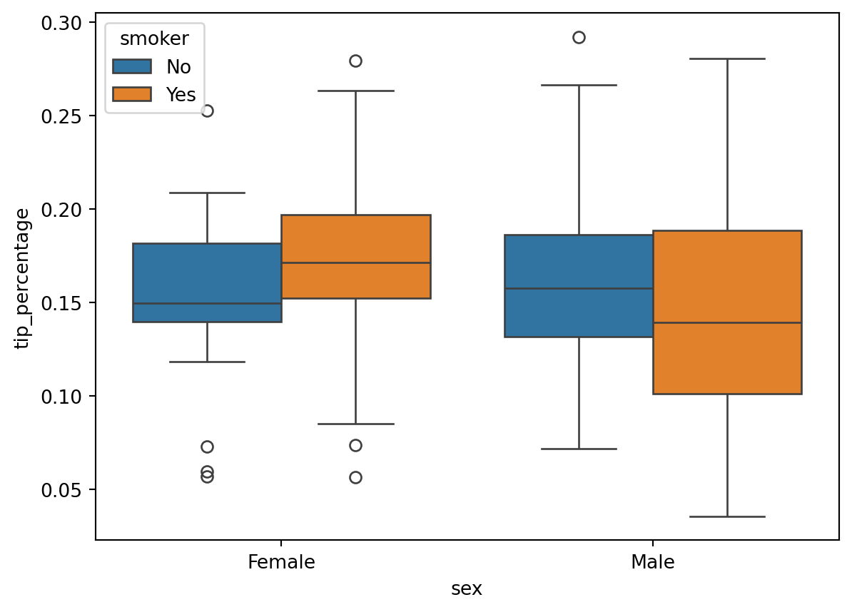

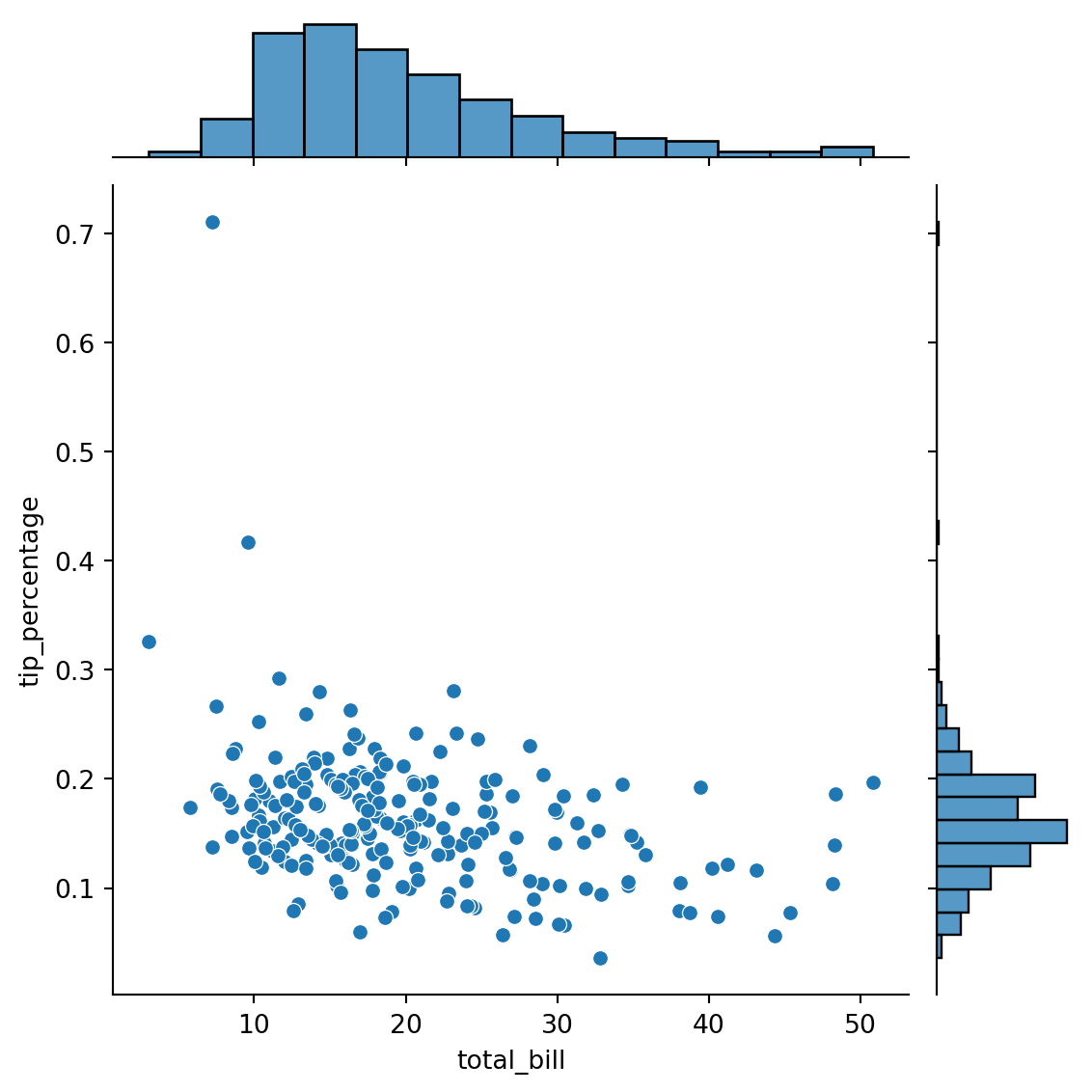
A jointplot (as in seaborn) is an enriched scatterplot with histograms on both axes.

When do customers go to this restaurant ?

Code

sns.countplot(x='day', hue="time", data=df)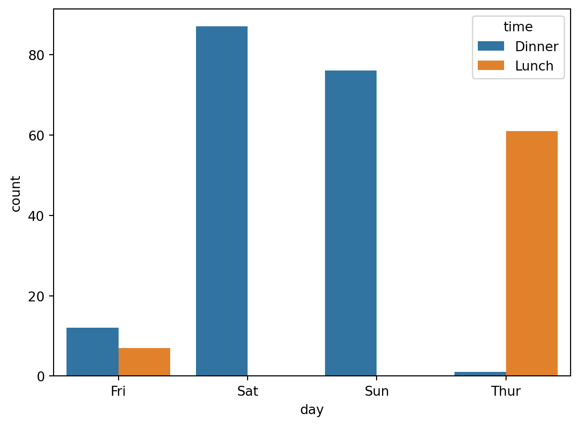

This is also called a barplot.

When do customers spend the most ?

Code

plt.figure(figsize=(7, 5))
sns.boxplot(x='day', y='total_bill', hue='time', data=df)
plt.legend(loc="upper left")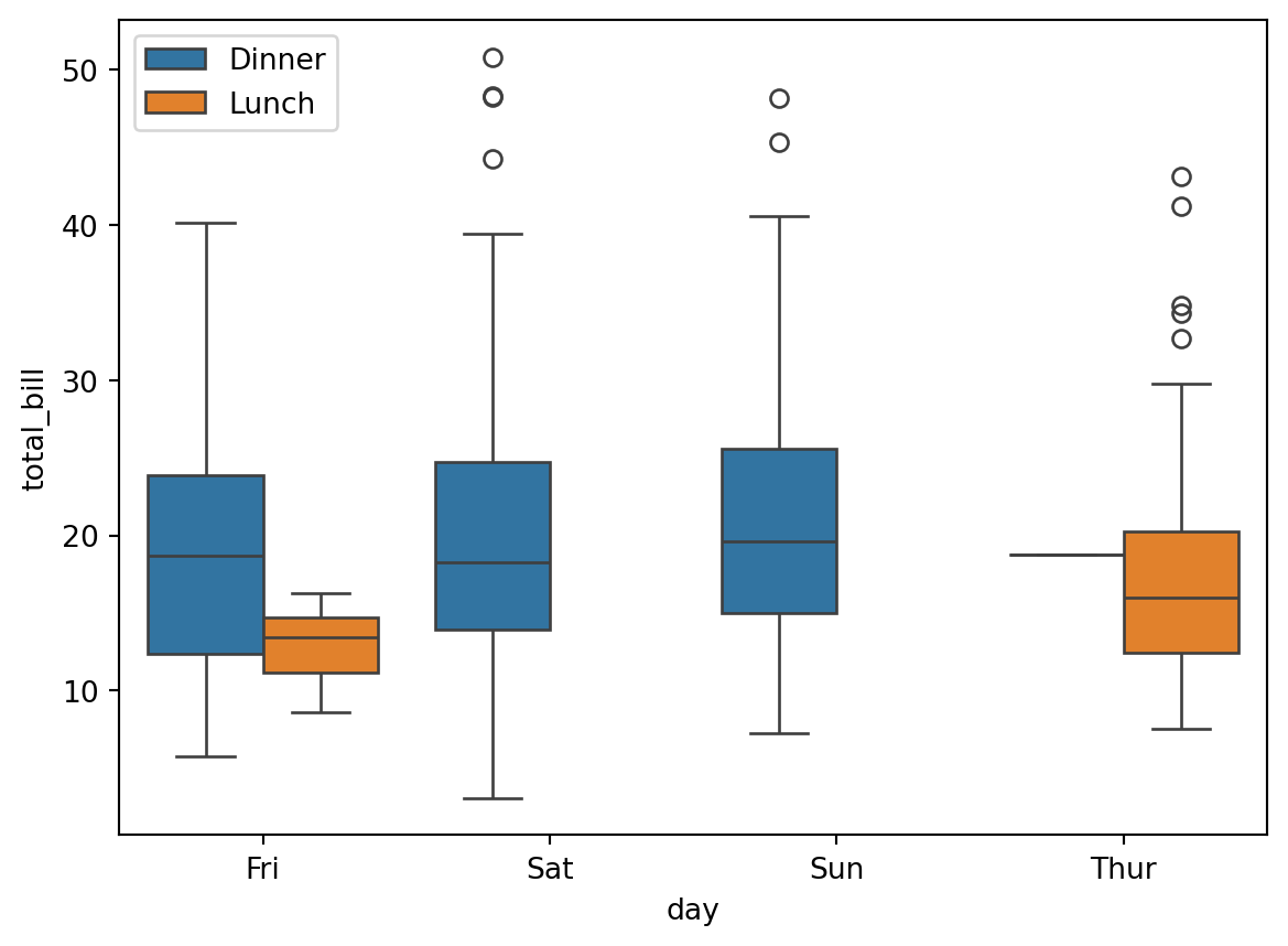

boxplot (box and whiskers plot) are used to sketch empirical distributions and to display summary statistics (median and quartiles).

Code

plt.figure(figsize=(7, 5))
sns.violinplot(x='day', y='total_bill', hue='time', split=True, data=df)
plt.legend(loc="upper left")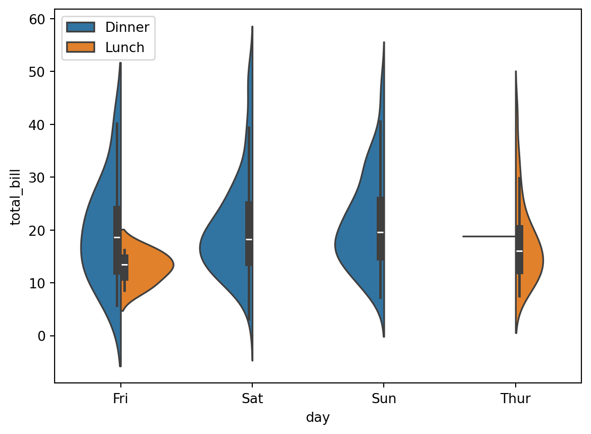

violinplot are sketchy variants of kernel density estimates.

Who spends the most ?

Code

sns.boxplot(x='sex', y='total_bill', hue='smoker', data=df)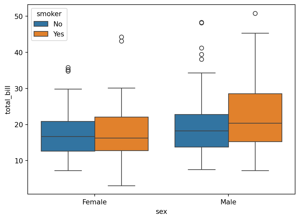

When should waiters want to work ?

Code

sns.boxplot(x='day', y='tip', hue='time', data=df)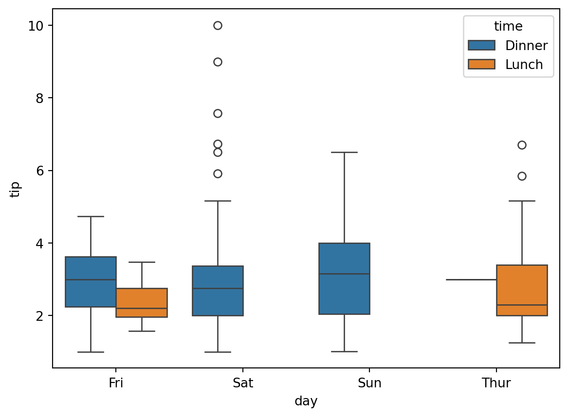

Code

sns.violinplot(x='day', y='tip', hue='time', data=df)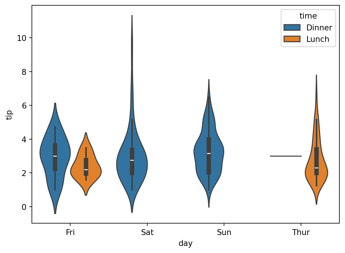

Data processing with `pandas`

Let us read again the tips.csv file

Code

import pandas as pd

dtypes = {
    "sex": "category",
    "smoker": "category",
    "day": "category",
    "time": "category"
} 

df = pd.read_csv("tips.csv", dtype=dtypes)
df.head()

	total_bill	tip	sex	smoker	day	time	size
0	16.99	1.01	Female	No	Sun	Dinner	2
1	10.34	1.66	Male	No	Sun	Dinner	3
2	21.01	3.50	Male	No	Sun	Dinner	3
3	23.68	3.31	Male	No	Sun	Dinner	2
4	24.59	3.61	Female	No	Sun	Dinner	4

Computations using `pandas` : broadcasting

Let’s add a column that contains the tip percentage. The content of this column is computed by performing elementwise operations between elements of two columns. This works as if the columns were NumPy arrays (even though they are not).

Code

df["tip_percentage"] = df["tip"] / df["total_bill"]
df.head()

	total_bill	tip	sex	smoker	day	time	size	tip_percentage
0	16.99	1.01	Female	No	Sun	Dinner	2	0.059447
1	10.34	1.66	Male	No	Sun	Dinner	3	0.160542
2	21.01	3.50	Male	No	Sun	Dinner	3	0.166587
3	23.68	3.31	Male	No	Sun	Dinner	2	0.139780
4	24.59	3.61	Female	No	Sun	Dinner	4	0.146808

The computation

```{python}
df["tip"] / df["total_bill"]
```

uses a broadcast rule (see NumPy notebook about broadcasting).

We can multiply, add, subtract, etc. together numpy arrays, Series or pandas dataframes when the computation makes sense in view of their respective shape

This principle is called broadcast or broadcasting.

Note

Broadcasting is a key feature of numpy ndarray, see

Code

df["tip"].shape, df["total_bill"].shape

((244,), (244,))

The tip and total_billcolumns have the same shape, so broadcasting performs pairwise division.

This corresponds to the following “hand-crafted” approach with a for loop:

#| 
for i in range(df.shape[0]):
    df.loc[i, "tip_percentage"] = df.loc[i, "tip"] / df.loc[i, "total_bill"]

But using such a loop is:

longer to write
less readable
prone to mistakes
and slower :(

NEVER use Python for-loops unless you need to !

Code

%%timeit -n 10
for i in range(df.shape[0]):
    df.loc[i, "tip_percentage"] = df.loc[i, "tip"] / df.loc[i, "total_bill"]

23.5 ms ± 133 μs per loop (mean ± std. dev. of 7 runs, 10 loops each)

Code

%%timeit -n 10
df["tip_percentage"] = df["tip"] / df["total_bill"]

67.9 μs ± 12.3 μs per loop (mean ± std. dev. of 7 runs, 10 loops each)

The for loop is \(\approx\) 100 times slower ! (even worse on larger data)

Pitfall. Changing values in a `DataFrame`

When you want to change a value in a DataFrame, never use

df["tip_percentage"].loc[i] = 42

but use

df.loc[i, "tip_percentage"] = 42

Caution

Use a single loc or iloc statement. The first version might not work: it might modify a copy of the column and not the dataframe itself !

Another example of broadcasting is:

Code

(100 * df[["tip_percentage"]]).head()

	tip_percentage
0	5.944673
1	16.054159
2	16.658734
3	13.978041
4	14.680765

where we multiplied each entry of the tip_percentage column by 100.

Remark

Note the difference between

df[['tip_percentage']]

which returns a DataFrame containing only the tip_percentage column and

df['tip_percentage']

which returns a Series containing the data of the tip_percentage column

Some more plots

How do the tip percentages relates to the total bill ?

Code

sns.jointplot(
    x="total_bill", 
    y="tip_percentage", 
    data=df
)

Who tips best ?

Code

sns.boxplot(
    x='sex', 
    y='tip_percentage', 
    hue='smoker', 
    data=df
)

Who tips best without the `tip_percentage` outliers ?

Code

sns.boxplot(
    x='sex', 
    y='tip_percentage', 
    hue='smoker', 
    data=df.loc[df["tip_percentage"] <= 0.3]
)

Object identity

Code

id(df)

123374907814880

The all-mighty `groupby` and `aggregate`

Many computations can be formulated as a groupby followed by and aggregation.

What is the mean `tip` and `tip percentage` each day ?

Code

df.head()

	total_bill	tip	sex	smoker	day	time	size	tip_percentage
0	16.99	1.01	Female	No	Sun	Dinner	2	0.059447
1	10.34	1.66	Male	No	Sun	Dinner	3	0.160542
2	21.01	3.50	Male	No	Sun	Dinner	3	0.166587
3	23.68	3.31	Male	No	Sun	Dinner	2	0.139780
4	24.59	3.61	Female	No	Sun	Dinner	4	0.146808

Code

try:
    (
        df
            .groupby("day", observed=True)
            .mean()
    )
except TypeError:
    print('TypeError: category dtype does not support aggregation "mean"')

TypeError: category dtype does not support aggregation "mean"

But we do not care about the size column here, so we can use instead

Code

(
    df[["total_bill", "tip", "tip_percentage", "day"]]
        .groupby("day")
        .mean()
)

/tmp/ipykernel_67207/1740663163.py:3: FutureWarning:

The default of observed=False is deprecated and will be changed to True in a future version of pandas. Pass observed=False to retain current behavior or observed=True to adopt the future default and silence this warning.

	total_bill	tip	tip_percentage
day
Fri	17.151579	2.734737	0.169913
Sat	20.441379	2.993103	0.153152
Sun	21.410000	3.255132	0.166897
Thur	17.682742	2.771452	0.161276

If we want to be more precise, we can groupby using several columns

Code

(
    df[["total_bill", "tip", "tip_percentage", "day", "time"]]   # selection
        .groupby(["day","time"])                                # partition
        .mean()                                                  # aggregation
)

/tmp/ipykernel_67207/391063870.py:3: FutureWarning:

The default of observed=False is deprecated and will be changed to True in a future version of pandas. Pass observed=False to retain current behavior or observed=True to adopt the future default and silence this warning.

		total_bill	tip	tip_percentage
day	time
Fri	Dinner	19.663333	2.940000	0.158916
Fri	Lunch	12.845714	2.382857	0.188765
Sat	Dinner	20.441379	2.993103	0.153152
Sat	Lunch	NaN	NaN	NaN
Sun	Dinner	21.410000	3.255132	0.166897
Sun	Lunch	NaN	NaN	NaN
Thur	Dinner	18.780000	3.000000	0.159744
Thur	Lunch	17.664754	2.767705	0.161301

Remarks

We obtain a DataFrame with a two-level indexing: on the day and the time
Groups must be homogeneous: we have NaN values for empty groups (e.g. Sat, Lunch)

Pro tip

Sometimes, it is more convenient to get the groups as columns instead of a multi-level index.

For this, use reset_index:

Code

(
    df[["total_bill", "tip", "tip_percentage", "day", "time"]]   # selection
        .groupby(["day", "time"])                                # partition
        .mean() # aggregation
        .reset_index()   # ako ungroup
)

/tmp/ipykernel_67207/835267922.py:3: FutureWarning:

The default of observed=False is deprecated and will be changed to True in a future version of pandas. Pass observed=False to retain current behavior or observed=True to adopt the future default and silence this warning.

	day	time	total_bill	tip	tip_percentage
0	Fri	Dinner	19.663333	2.940000	0.158916
1	Fri	Lunch	12.845714	2.382857	0.188765
2	Sat	Dinner	20.441379	2.993103	0.153152
3	Sat	Lunch	NaN	NaN	NaN
4	Sun	Dinner	21.410000	3.255132	0.166897
5	Sun	Lunch	NaN	NaN	NaN
6	Thur	Dinner	18.780000	3.000000	0.159744
7	Thur	Lunch	17.664754	2.767705	0.161301

Another pro tip: care about code readers

Computations with pandas can include many operations that are pipelined until the final computation.

Pipelining many operations is good practice and perfectly normal, but in order to make the code readable you can put it between parenthesis (python expression) as follows:

Code

(
    df[["total_bill", "tip", "tip_percentage", "day", "time"]]
    .groupby(["day", "time"])
    .mean()
    .reset_index()
    # and on top of all this we sort the dataframe with respect 
    # to the tip_percentage
    .sort_values("tip_percentage")
)

/tmp/ipykernel_67207/45053252.py:3: FutureWarning:

The default of observed=False is deprecated and will be changed to True in a future version of pandas. Pass observed=False to retain current behavior or observed=True to adopt the future default and silence this warning.

	day	time	total_bill	tip	tip_percentage
2	Sat	Dinner	20.441379	2.993103	0.153152
0	Fri	Dinner	19.663333	2.940000	0.158916
6	Thur	Dinner	18.780000	3.000000	0.159744
7	Thur	Lunch	17.664754	2.767705	0.161301
4	Sun	Dinner	21.410000	3.255132	0.166897
1	Fri	Lunch	12.845714	2.382857	0.188765
3	Sat	Lunch	NaN	NaN	NaN
5	Sun	Lunch	NaN	NaN	NaN

Displaying a `DataFrame` with `style`

Now, we can answer, with style, to the question: what are the average tip percentages along the week ?

Code

(
    df[["tip_percentage", "day", "time"]]
    .groupby(["day", "time"])
    .mean()
    # At the end of the pipeline you can use .style
    .style
    # Print numerical values as percentages 
    .format("{:.2%}")
    .background_gradient()
)

/tmp/ipykernel_67207/838795167.py:3: FutureWarning:

The default of observed=False is deprecated and will be changed to True in a future version of pandas. Pass observed=False to retain current behavior or observed=True to adopt the future default and silence this warning.

		tip_percentage
day	time
Fri	Dinner	15.89%
Fri	Lunch	18.88%
Sat	Dinner	15.32%
Sat	Lunch	nan%
Sun	Dinner	16.69%
Sun	Lunch	nan%
Thur	Dinner	15.97%
Thur	Lunch	16.13%

Removing the `NaN` values

But the NaN values are somewhat annoying. Let’s remove them

Code

(
    df[["tip_percentage", "day", "time"]]
    .groupby(["day", "time"])
    .mean()
    # We just add this from the previous pipeline
    .dropna()
    .style
    .format("{:.2%}")
    .background_gradient()
)

/tmp/ipykernel_67207/2662169510.py:3: FutureWarning:

The default of observed=False is deprecated and will be changed to True in a future version of pandas. Pass observed=False to retain current behavior or observed=True to adopt the future default and silence this warning.

		tip_percentage
day	time
Fri	Dinner	15.89%
Fri	Lunch	18.88%
Sat	Dinner	15.32%
Sun	Dinner	16.69%
Thur	Dinner	15.97%
Thur	Lunch	16.13%

Now, we see when tip_percentage is maximal. But what about the standard deviation?

We used only .mean() for now, but we can use several aggregating function using .agg()

Code

(
    df[["tip_percentage", "day", "time"]]
    .groupby(["day", "time"])
    .agg(["mean", "std"])   # we feed `agg`  with a list of names of callables 
    .dropna()
    .style
    .format("{:.2%}")
    .background_gradient()
)

/tmp/ipykernel_67207/3957220442.py:3: FutureWarning:

The default of observed=False is deprecated and will be changed to True in a future version of pandas. Pass observed=False to retain current behavior or observed=True to adopt the future default and silence this warning.

		tip_percentage
		mean	std
day	time
Fri	Dinner	15.89%	4.70%
Fri	Lunch	18.88%	4.59%
Sat	Dinner	15.32%	5.13%
Sun	Dinner	16.69%	8.47%
Thur	Lunch	16.13%	3.90%

And we can use also .describe() as aggregation function. Moreover we - use the subset option to specify which column we want to style - we use ("tip_percentage", "count") to access multi-level index

Code

(
    df[["tip_percentage", "day", "time"]]
    .groupby(["day", "time"])
    .describe()    # all-purpose summarising function
)

/tmp/ipykernel_67207/3924876303.py:3: FutureWarning:

The default of observed=False is deprecated and will be changed to True in a future version of pandas. Pass observed=False to retain current behavior or observed=True to adopt the future default and silence this warning.

		tip_percentage
		count	mean	std	min	25%	50%	75%	max
day	time
Fri	Dinner	12.0	0.158916	0.047024	0.103555	0.123613	0.144742	0.179199	0.263480
Fri	Lunch	7.0	0.188765	0.045885	0.117735	0.167289	0.187735	0.210996	0.259314
Sat	Dinner	87.0	0.153152	0.051293	0.035638	0.123863	0.151832	0.188271	0.325733
Sun	Dinner	76.0	0.166897	0.084739	0.059447	0.119982	0.161103	0.187889	0.710345
Thur	Dinner	1.0	0.159744	NaN	0.159744	0.159744	0.159744	0.159744	0.159744
Thur	Lunch	61.0	0.161301	0.038972	0.072961	0.137741	0.153846	0.193424	0.266312

Code

(
    df[["tip_percentage", "day", "time"]]
    .groupby(["day", "time"])
    .describe()
    .dropna()
    .style
    .bar(subset=[("tip_percentage", "count")])
    .background_gradient(subset=[("tip_percentage", "50%")])
)

/tmp/ipykernel_67207/673231177.py:3: FutureWarning:

The default of observed=False is deprecated and will be changed to True in a future version of pandas. Pass observed=False to retain current behavior or observed=True to adopt the future default and silence this warning.

		tip_percentage
		count	mean	std	min	25%	50%	75%	max
day	time
Fri	Dinner	12.000000	0.158916	0.047024	0.103555	0.123613	0.144742	0.179199	0.263480
Fri	Lunch	7.000000	0.188765	0.045885	0.117735	0.167289	0.187735	0.210996	0.259314
Sat	Dinner	87.000000	0.153152	0.051293	0.035638	0.123863	0.151832	0.188271	0.325733
Sun	Dinner	76.000000	0.166897	0.084739	0.059447	0.119982	0.161103	0.187889	0.710345
Thur	Lunch	61.000000	0.161301	0.038972	0.072961	0.137741	0.153846	0.193424	0.266312

Supervised learning of `tip` based on the `total_bill`

As an example of very simple machine-learning problem, let us try to understand how we can predict tip based on total_bill.

Code

import numpy as np

plt.scatter(df["total_bill"], df["tip"])
plt.xlabel("total_bill", fontsize=12)
plt.ylabel("tip", fontsize=12)

Text(0, 0.5, 'tip')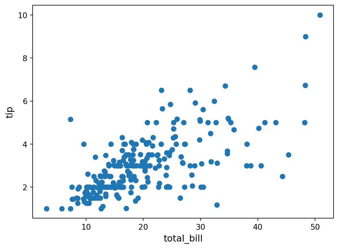

There’s a rough linear dependence between the two. Let us try to find it by hand!
Namely, we look for numbers \(b\) and \(w\) such that

tip ≈ b + w × total_bill

for all the examples of pairs of (tip, total_bill) we observe in the data.

In machine learning, we say that this is a very simple example of a supervised learning problem (here it is a regression problem), where tip is the label and where total_bill is the (only) feature, for which we intend to use a linear predictor.

Code

plt.scatter(df["total_bill"], df["tip"])
plt.xlabel("total_bill", fontsize=12)
plt.ylabel("tip", fontsize=12)

slope = 1.0
intercept = 0.0

x = np.linspace(0, 50, 1000)
plt.plot(x, intercept + slope * x, color="red")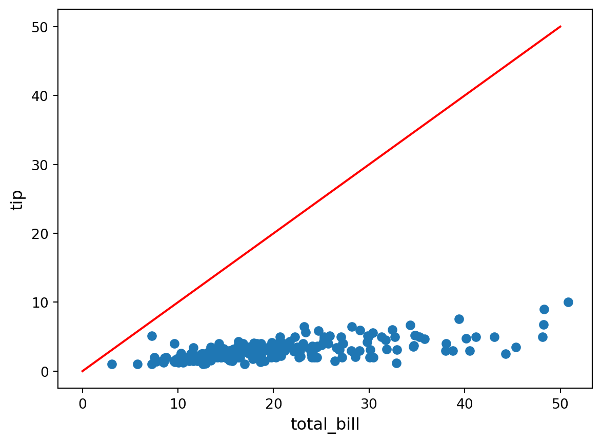

A more interactive way

This might require

Code

!pip install ipympl

Requirement already satisfied: ipympl in /home/boucheron/Documents/IFEBY310/.venv/lib/python3.12/site-packages (0.9.5)
Requirement already satisfied: ipython<9 in /home/boucheron/Documents/IFEBY310/.venv/lib/python3.12/site-packages (from ipympl) (8.31.0)
Requirement already satisfied: ipywidgets<9,>=7.6.0 in /home/boucheron/Documents/IFEBY310/.venv/lib/python3.12/site-packages (from ipympl) (8.1.5)
Requirement already satisfied: matplotlib<4,>=3.4.0 in /home/boucheron/Documents/IFEBY310/.venv/lib/python3.12/site-packages (from ipympl) (3.10.0)
Requirement already satisfied: numpy in /home/boucheron/Documents/IFEBY310/.venv/lib/python3.12/site-packages (from ipympl) (2.4.0)
Requirement already satisfied: pillow in /home/boucheron/Documents/IFEBY310/.venv/lib/python3.12/site-packages (from ipympl) (11.0.0)
Requirement already satisfied: traitlets<6 in /home/boucheron/Documents/IFEBY310/.venv/lib/python3.12/site-packages (from ipympl) (5.14.3)
Requirement already satisfied: decorator in /home/boucheron/Documents/IFEBY310/.venv/lib/python3.12/site-packages (from ipython<9->ipympl) (5.1.1)
Requirement already satisfied: jedi>=0.16 in /home/boucheron/Documents/IFEBY310/.venv/lib/python3.12/site-packages (from ipython<9->ipympl) (0.19.2)
Requirement already satisfied: matplotlib-inline in /home/boucheron/Documents/IFEBY310/.venv/lib/python3.12/site-packages (from ipython<9->ipympl) (0.1.7)
Requirement already satisfied: pexpect>4.3 in /home/boucheron/Documents/IFEBY310/.venv/lib/python3.12/site-packages (from ipython<9->ipympl) (4.9.0)
Requirement already satisfied: prompt_toolkit<3.1.0,>=3.0.41 in /home/boucheron/Documents/IFEBY310/.venv/lib/python3.12/site-packages (from ipython<9->ipympl) (3.0.48)
Requirement already satisfied: pygments>=2.4.0 in /home/boucheron/Documents/IFEBY310/.venv/lib/python3.12/site-packages (from ipython<9->ipympl) (2.18.0)
Requirement already satisfied: stack_data in /home/boucheron/Documents/IFEBY310/.venv/lib/python3.12/site-packages (from ipython<9->ipympl) (0.6.3)
Requirement already satisfied: comm>=0.1.3 in /home/boucheron/Documents/IFEBY310/.venv/lib/python3.12/site-packages (from ipywidgets<9,>=7.6.0->ipympl) (0.2.2)
Requirement already satisfied: widgetsnbextension~=4.0.12 in /home/boucheron/Documents/IFEBY310/.venv/lib/python3.12/site-packages (from ipywidgets<9,>=7.6.0->ipympl) (4.0.13)
Requirement already satisfied: jupyterlab-widgets~=3.0.12 in /home/boucheron/Documents/IFEBY310/.venv/lib/python3.12/site-packages (from ipywidgets<9,>=7.6.0->ipympl) (3.0.16)
Requirement already satisfied: contourpy>=1.0.1 in /home/boucheron/Documents/IFEBY310/.venv/lib/python3.12/site-packages (from matplotlib<4,>=3.4.0->ipympl) (1.3.1)
Requirement already satisfied: cycler>=0.10 in /home/boucheron/Documents/IFEBY310/.venv/lib/python3.12/site-packages (from matplotlib<4,>=3.4.0->ipympl) (0.12.1)
Requirement already satisfied: fonttools>=4.22.0 in /home/boucheron/Documents/IFEBY310/.venv/lib/python3.12/site-packages (from matplotlib<4,>=3.4.0->ipympl) (4.55.3)
Requirement already satisfied: kiwisolver>=1.3.1 in /home/boucheron/Documents/IFEBY310/.venv/lib/python3.12/site-packages (from matplotlib<4,>=3.4.0->ipympl) (1.4.8)
Requirement already satisfied: packaging>=20.0 in /home/boucheron/Documents/IFEBY310/.venv/lib/python3.12/site-packages (from matplotlib<4,>=3.4.0->ipympl) (24.2)
Requirement already satisfied: pyparsing>=2.3.1 in /home/boucheron/Documents/IFEBY310/.venv/lib/python3.12/site-packages (from matplotlib<4,>=3.4.0->ipympl) (3.2.1)
Requirement already satisfied: python-dateutil>=2.7 in /home/boucheron/Documents/IFEBY310/.venv/lib/python3.12/site-packages (from matplotlib<4,>=3.4.0->ipympl) (2.9.0.post0)
Requirement already satisfied: wcwidth in /home/boucheron/Documents/IFEBY310/.venv/lib/python3.12/site-packages (from prompt_toolkit<3.1.0,>=3.0.41->ipython<9->ipympl) (0.2.13)
Requirement already satisfied: parso<0.9.0,>=0.8.4 in /home/boucheron/Documents/IFEBY310/.venv/lib/python3.12/site-packages (from jedi>=0.16->ipython<9->ipympl) (0.8.4)
Requirement already satisfied: ptyprocess>=0.5 in /home/boucheron/Documents/IFEBY310/.venv/lib/python3.12/site-packages (from pexpect>4.3->ipython<9->ipympl) (0.7.0)
Requirement already satisfied: six>=1.5 in /home/boucheron/Documents/IFEBY310/.venv/lib/python3.12/site-packages (from python-dateutil>=2.7->matplotlib<4,>=3.4.0->ipympl) (1.17.0)
Requirement already satisfied: executing>=1.2.0 in /home/boucheron/Documents/IFEBY310/.venv/lib/python3.12/site-packages (from stack_data->ipython<9->ipympl) (2.1.0)
Requirement already satisfied: asttokens>=2.1.0 in /home/boucheron/Documents/IFEBY310/.venv/lib/python3.12/site-packages (from stack_data->ipython<9->ipympl) (3.0.0)
Requirement already satisfied: pure-eval in /home/boucheron/Documents/IFEBY310/.venv/lib/python3.12/site-packages (from stack_data->ipython<9->ipympl) (0.2.3)

Code

import ipywidgets as widgets
import matplotlib.pyplot as plt
import numpy as np

%matplotlib widget
%matplotlib inline

x = np.linspace(0, 50, 1000)

@widgets.interact(intercept=(-5, 5, 1.), slope=(0, 1, .05))
def update(intercept=0.0, slope=0.5):
    plt.scatter(df["total_bill"], df["tip"])
    plt.plot(x, intercept + slope * x, color="red")
    plt.xlim((0, 50))
    plt.ylim((0, 10))
    plt.xlabel("total_bill", fontsize=12)
    plt.ylabel("tip", fontsize=12)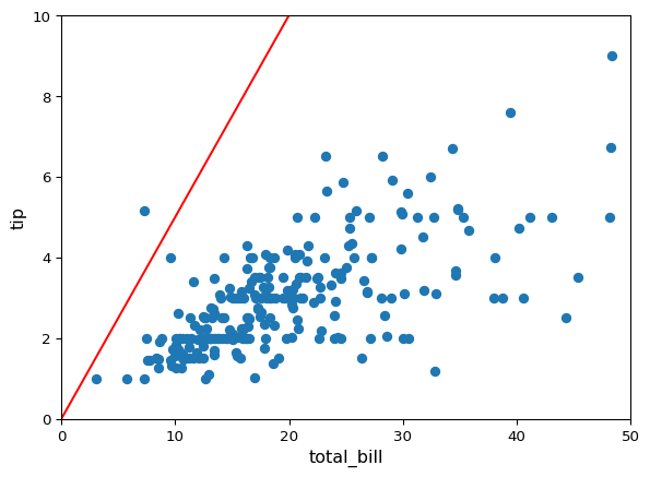

This is kind of tedious to do this by hand… it would be nice to come up with an automated way of doing this. Moreover:

We are using a linear function, while something more complicated (such as a polynomial) might be better
More importantly, we use only the total_bill column to predict the tip, while we know about many other things

Code

df.head()

	total_bill	tip	sex	smoker	day	time	size	tip_percentage
0	16.99	1.01	Female	No	Sun	Dinner	2	0.059447
1	10.34	1.66	Male	No	Sun	Dinner	3	0.160542
2	21.01	3.50	Male	No	Sun	Dinner	3	0.166587
3	23.68	3.31	Male	No	Sun	Dinner	2	0.139780
4	24.59	3.61	Female	No	Sun	Dinner	4	0.146808

One-hot encoding of categorical variables

We can’t perform computations (products and sums) with columns containing categorical variables. So, we can’t use them like this to predict the tip. We need to convert them to numbers somehow.

The most classical approach for this is one-hot encoding (or “create dummies” or “binarize”) of the categorical variables, which can be easily achieved with pandas.get_dummies

Why one-hot ? See wikipedia for a plausible explanation

Code

df_one_hot = pd.get_dummies(df, prefix_sep='#')
df_one_hot.head(5)

	total_bill	tip	size	tip_percentage	sex#Female	sex#Male	smoker#No	smoker#Yes	day#Fri	day#Sat	day#Sun	day#Thur	time#Dinner	time#Lunch
0	16.99	1.01	2	0.059447	True	False	True	False	False	False	True	False	True	False
1	10.34	1.66	3	0.160542	False	True	True	False	False	False	True	False	True	False
2	21.01	3.50	3	0.166587	False	True	True	False	False	False	True	False	True	False
3	23.68	3.31	2	0.139780	False	True	True	False	False	False	True	False	True	False
4	24.59	3.61	4	0.146808	True	False	True	False	False	False	True	False	True	False

Only the categorical columns have been one-hot encoded. For instance, the "day" column is replaced by 4 columns named "day#Thur", "day#Fri", "day#Sat", "day#Sun", since "day" has 4 modalities (see next line).

Code

df['day'].unique()

['Sun', 'Sat', 'Thur', 'Fri']
Categories (4, object): ['Fri', 'Sat', 'Sun', 'Thur']

Code

df_one_hot.dtypes

total_bill        float64
tip               float64
size                int64
tip_percentage    float64
sex#Female           bool
sex#Male             bool
smoker#No            bool
smoker#Yes           bool
day#Fri              bool
day#Sat              bool
day#Sun              bool
day#Thur             bool
time#Dinner          bool
time#Lunch           bool
dtype: object

Pitfall. Colinearities with one-hot encoding

Sums over dummies for sex, smoker, day, time and size are all equal to one (by constrution of the one-hot encoded vectors).

Leads to colinearities in the matrix of features
It is much harder to train a linear regressor when the columns of the features matrix has colinearities

Code

day_cols = [col for col in df_one_hot.columns if col.startswith("day")]
df_one_hot[day_cols].head()
df_one_hot[day_cols].sum(axis=1)

0      1
1      1
2      1
3      1
4      1
      ..
239    1
240    1
241    1
242    1
243    1
Length: 244, dtype: int64

Code

all(df_one_hot[day_cols].sum(axis=1) == 1)

True

The most standard solution is to remove a modality (i.e. remove a one-hot encoding vector). Simply achieved by specifying drop_first=True in the get_dummies function.

Code

df["day"].unique()

['Sun', 'Sat', 'Thur', 'Fri']
Categories (4, object): ['Fri', 'Sat', 'Sun', 'Thur']

Code

pd.get_dummies(df, prefix_sep='#', drop_first=True).head()

	total_bill	tip	size	tip_percentage	sex#Male	smoker#Yes	day#Sat	day#Sun	day#Thur	time#Lunch
0	16.99	1.01	2	0.059447	False	False	False	True	False	False
1	10.34	1.66	3	0.160542	True	False	False	True	False	False
2	21.01	3.50	3	0.166587	True	False	False	True	False	False
3	23.68	3.31	2	0.139780	True	False	False	True	False	False
4	24.59	3.61	4	0.146808	False	False	False	True	False	False

Now, if a categorical feature has \(K\) modalities/levels, we use only \(K-1\) dummies. For instance, there is no more sex#Female binary column.

Question. So, a linear regression won’t fit a weight for sex#Female. But, where do the model weights of the dropped binary columns go ?

Answer. They just “go” to the intercept: interpretation of the population bias depends on the “dropped” one-hot encodings.

So, we actually fit:

\[ \begin{array}{rl} \texttt{tip} \approx b & + w_1 \times \texttt{total\_bill} + w_2 \times \texttt{size} \\ & + w_3 \times \texttt{sex\#Male} + w_4 \times \texttt{smoker\#Yes} \\ & + w_5 \times \texttt{day\#Sat} + w_6 \times \texttt{day\#Sun} + w_7 \times \texttt{day\#Thur} \\ & + w_8 \times \texttt{time\#Lunch} \end{array} \]

Why ?

Why (con’t) ?

Where ?

Core components of pandas

Creating a DataFrame from scratch

Indexing

.loc versus .iloc

Main attributes and methods of a DataFrame

Missing values

Adding a column

Adding a column with the date

Casting a Series to another type

Handling errors during conversion

Slices and subsets of rows or columns

Write our data to a CSV file

Reading data and working with it

The category type

Computing statistics

Plotting backends for Pandas DataFrames

Setting the plotting backend

Using different backends

Matplotlib (default)

Plotly backend

Per-plot backend selection

Data visualization with matplotlib and seaborn

How do the tip depends on the total bill ?

When do customers go to this restaurant ?

When do customers spend the most ?

Who spends the most ?

When should waiters want to work ?

Data processing with pandas

Computations using pandas : broadcasting

Pitfall. Changing values in a DataFrame

Some more plots

How do the tip percentages relates to the total bill ?

Who tips best ?

Who tips best without the tip_percentage outliers ?

The all-mighty groupby and aggregate

What is the mean tip and tip percentage each day ?

Pro tip

Another pro tip: care about code readers

Displaying a DataFrame with style

Removing the NaN values

Supervised learning of tip based on the total_bill

A more interactive way

One-hot encoding of categorical variables

Pitfall. Colinearities with one-hot encoding

Creating a `DataFrame` from scratch

`.loc` versus `.iloc`

Main attributes and methods of a `DataFrame`

The `category` type

Data visualization with `matplotlib` and `seaborn`

Data processing with `pandas`

Computations using `pandas` : broadcasting

Pitfall. Changing values in a `DataFrame`

Who tips best without the `tip_percentage` outliers ?

The all-mighty `groupby` and `aggregate`

What is the mean `tip` and `tip percentage` each day ?

Displaying a `DataFrame` with `style`

Removing the `NaN` values

Supervised learning of `tip` based on the `total_bill`