Hierarchical Clustering

Analyse de Données Master MIDS

Équipe EAD

LPSM Université Paris-Cité

2025-04-02

Roadmap

• Hierarchical clustering
• Inside hclust
• Comparing dendrograms
• The End

Hierarchical clustering

• Dendrogram : what is it?
• From dendrogram to clusterings: cutting a dendrogram
• Grow a dendrogram
• Displaying a dendrogram
• Validation and assesment

Hierarchical clustering […] is a method of cluster analysis which seeks to build a hierarchy of clusters

from Wikipedia

Recall that a clustering is a partition of some dataset

A partition \(D\) of \(\mathcal{X}\) is a refinement of another partition \(D'\) if every class in \(D\) is a subset of a class in \(D'\). Partitions \(D\) and \(D'\) are said to be nested

A hierarchical clustering of \(\mathcal{X}\) is a sequence of \(|\mathcal{X}|\) nested partitions of \(\mathcal{X}\), starting from the trivial partition into \(|\mathcal{X}|\) singletons and ending into the trivial partition in \(1\) subset ( \(\mathcal{X}\) itself)

A hierarchical clustering consists of \(|\mathcal{X}|\) nested flat clusterings

We will explore agglomerative or bottom-up methods to build hierarchical clusterings

Hierchical clustering and dendrogram

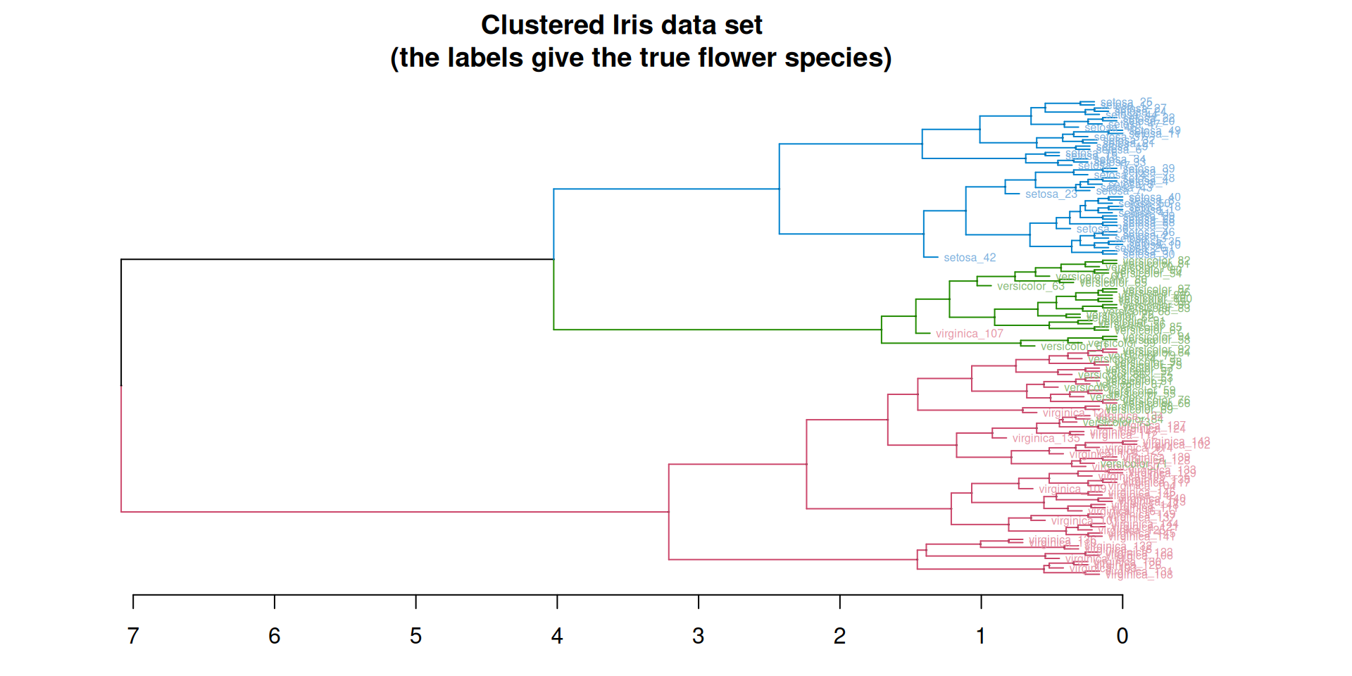
The result of hierarchical clustering is a tree where leafs are labelled by sample points and internal nodes correspond to merging operations

The tree conveys more information: if the tree is properly decorated, it is possible to reconstruct the different merging steps and to know which rule was applied when some merging operation was performed

The tree is called a dendrogram

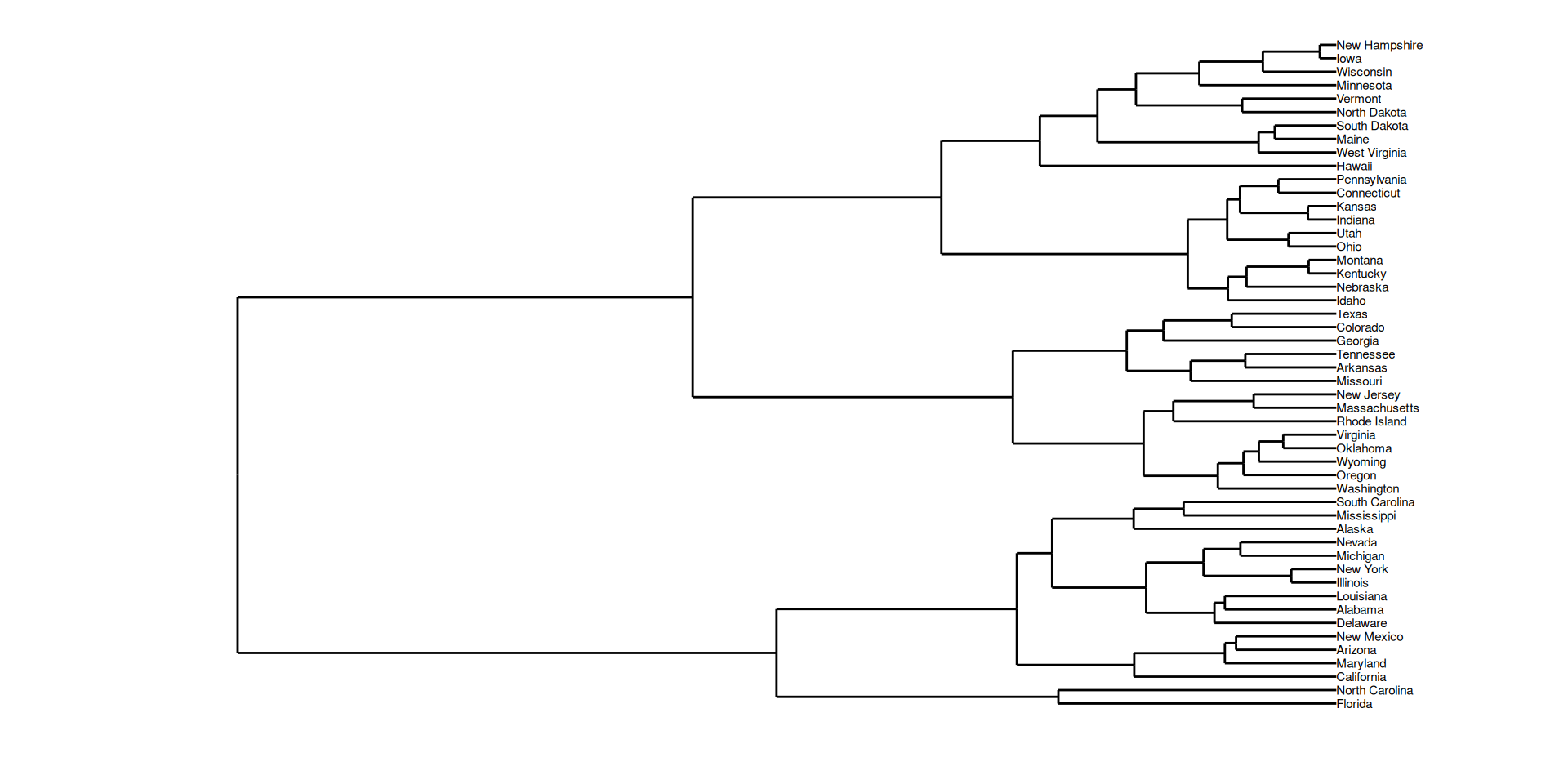
Violent Crime Rates by US State

Description

This data set contains statistics, in arrests per 100,000 residents for assault, murder, and rape in each of the 50 US states in 1973. Also given is the percent of the population living in urban areas.

Dendrogram and trees show up in several areas.

Classification and Regression trees play an important role in Machine Learning.

ggdendro and dendextend may also be used to manipulate regression trees

• Cutting a dendrogram: getting a flat clustering

• Building a dendrogram: inside hclust

• Displaying, reporting dendrograms

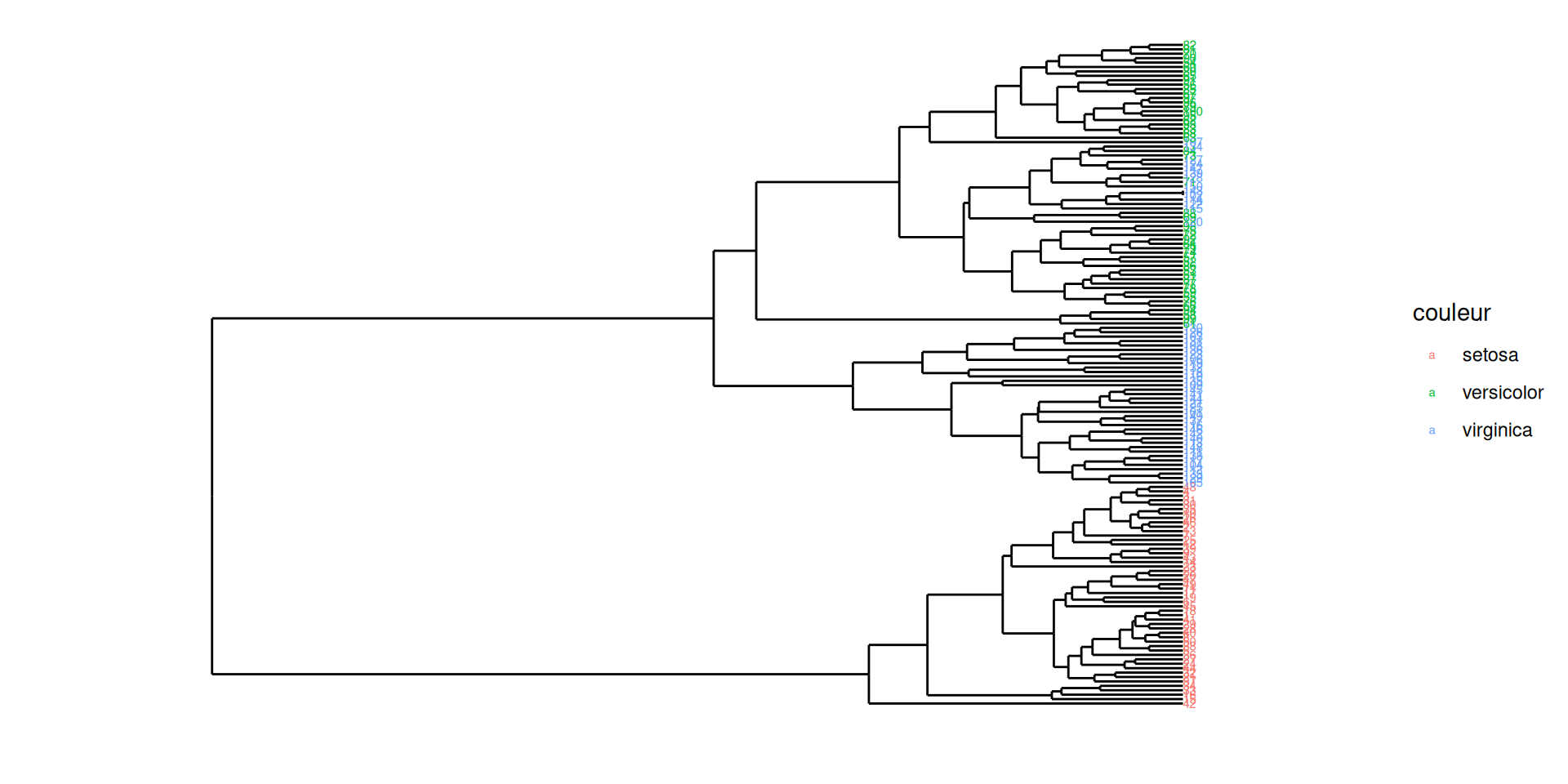
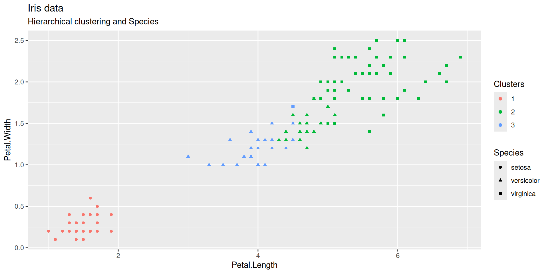
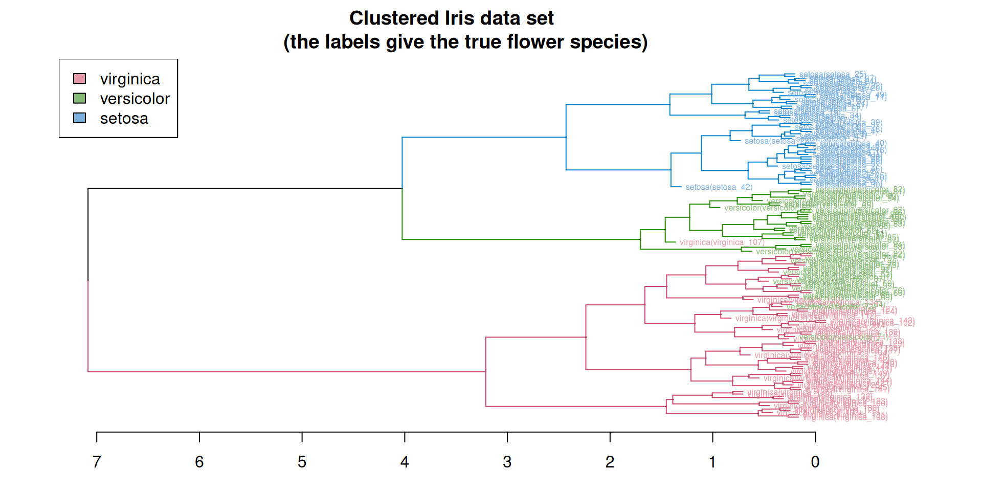
Cutting a dendrogram: Iris illustration

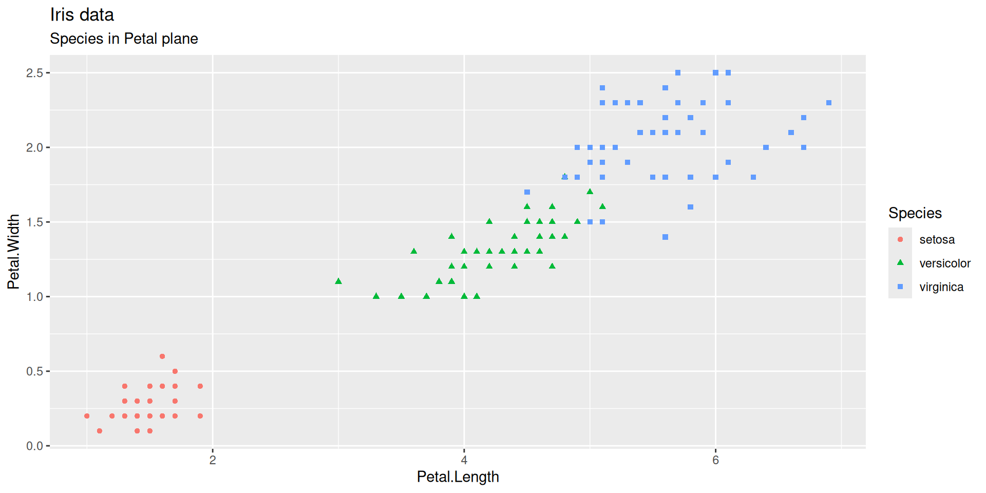
The famous (Fisher’s or Anderson’s) iris data set gives the measurements in centimeters of the variables sepal length and width and petal length and width, respectively, for 50 flowers from each of 3 species of iris. The species are Iris setosa, versicolor, and virginica.

The Iris flower data set is fun for learning supervised classification algorithms, and is known as a difficult case for unsupervised learning.

The Setosa species are distinctly different from Versicolor and Virginica (they have lower petal length and width). But Versicolor and Virginica cannot easily be separated based on measurements of their sepal and petal width/length.

<ScaleContinuousPosition>
 Range:  
 Limits:    0 --    1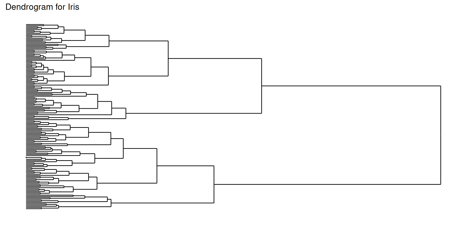

• as.matrix(dist(iris[,1:4])) returns the matrix of pairwise distances
• Default distance is Euclidean distance
• What about using broom::augment?
• There is no augment.hclust method: No augment method for objects of class hclust

:::

hclust pipeline

dendro_iris <- iris |> 
  select(where(is.numeric)) |>  
  dist() |> 
  hclust() |> 
  dendro_data() 

mydendro <- . %$% {  #<<
  ggplot() + 
    geom_segment(
      data = segments,   #<<
      aes(
        x = x, y = y, 
        xend = xend, 
        yend = yend)
  ) +
  geom_text(
    data = labels, #<<
    aes(
      x = x, y = y, 
      label = label, hjust = 0),
    size = 2
  ) +
  coord_flip() +
  scale_y_reverse(expand = c(0.2, 0)) +
  theme_dendro()  
}

mydendro(dendro_iris)

Inside ggdendro

What is an object of class dendro made of?

It a list of four elements:

• segments
• labels
• leaf_labels
• class

Element segments is a data frame with four columns. Each row represent a segment that is part of a graphical representation of the hierarchy. There are horizontal and vertical segments

Element labels is used to label the tree leafs.

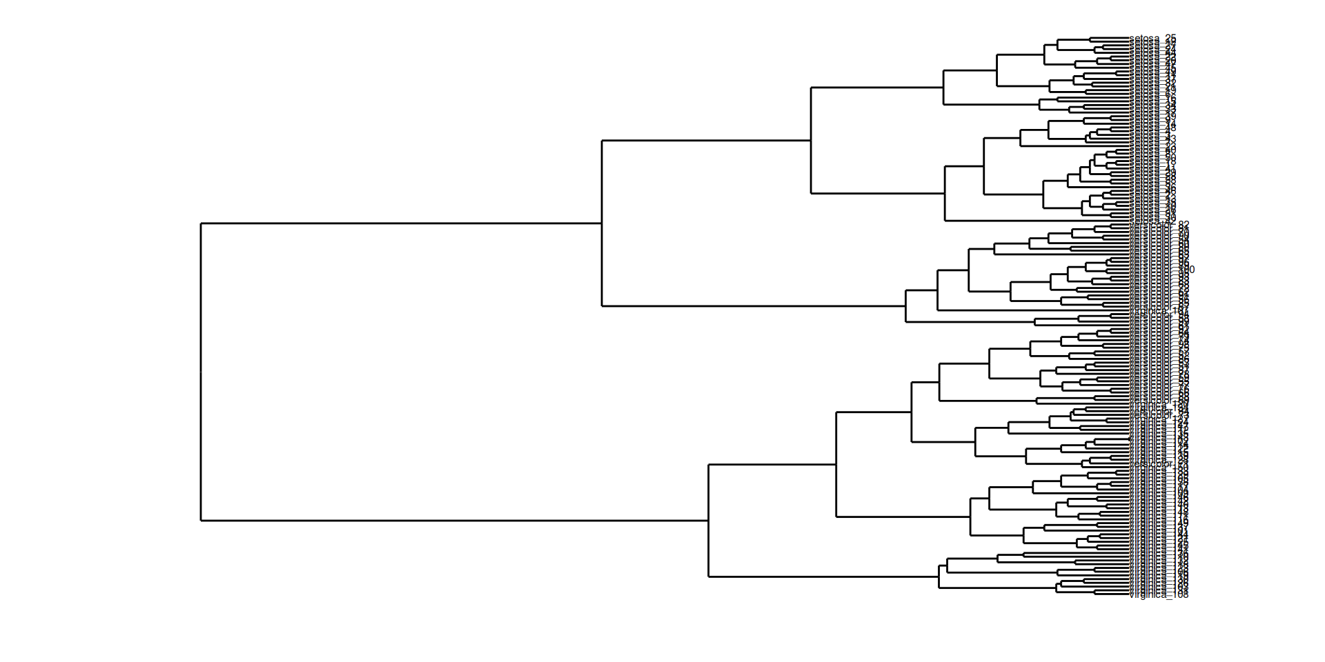
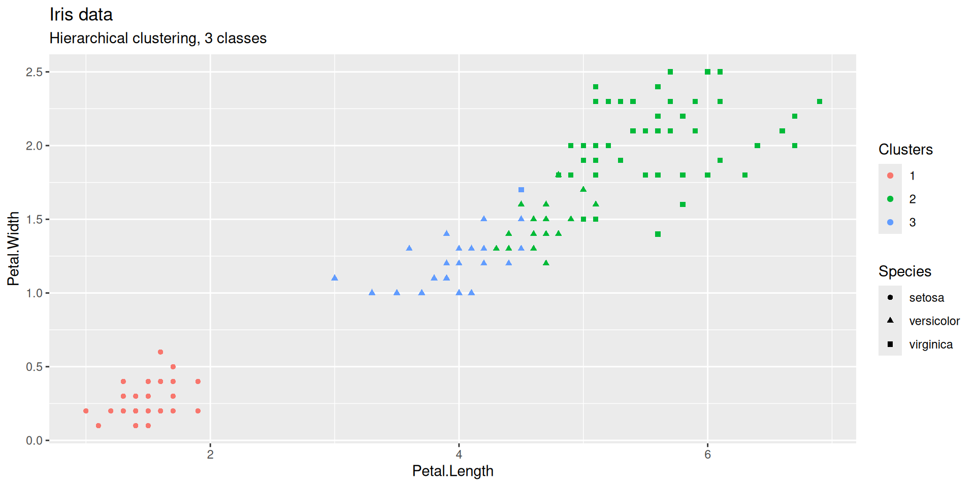
Cutting a dendrogram: Iris illustration (continued)

p <- iris %>%
  ggplot() +
  aes(x=Petal.Length, y=Petal.Width)

p +
  geom_point(
    aes(
      shape=Species, 
      colour=Species)
  ) +
# labs(shape= "Species") +
  ggtitle(
    label= "Iris data",
    subtitle = "Species in Petal plane"
  )

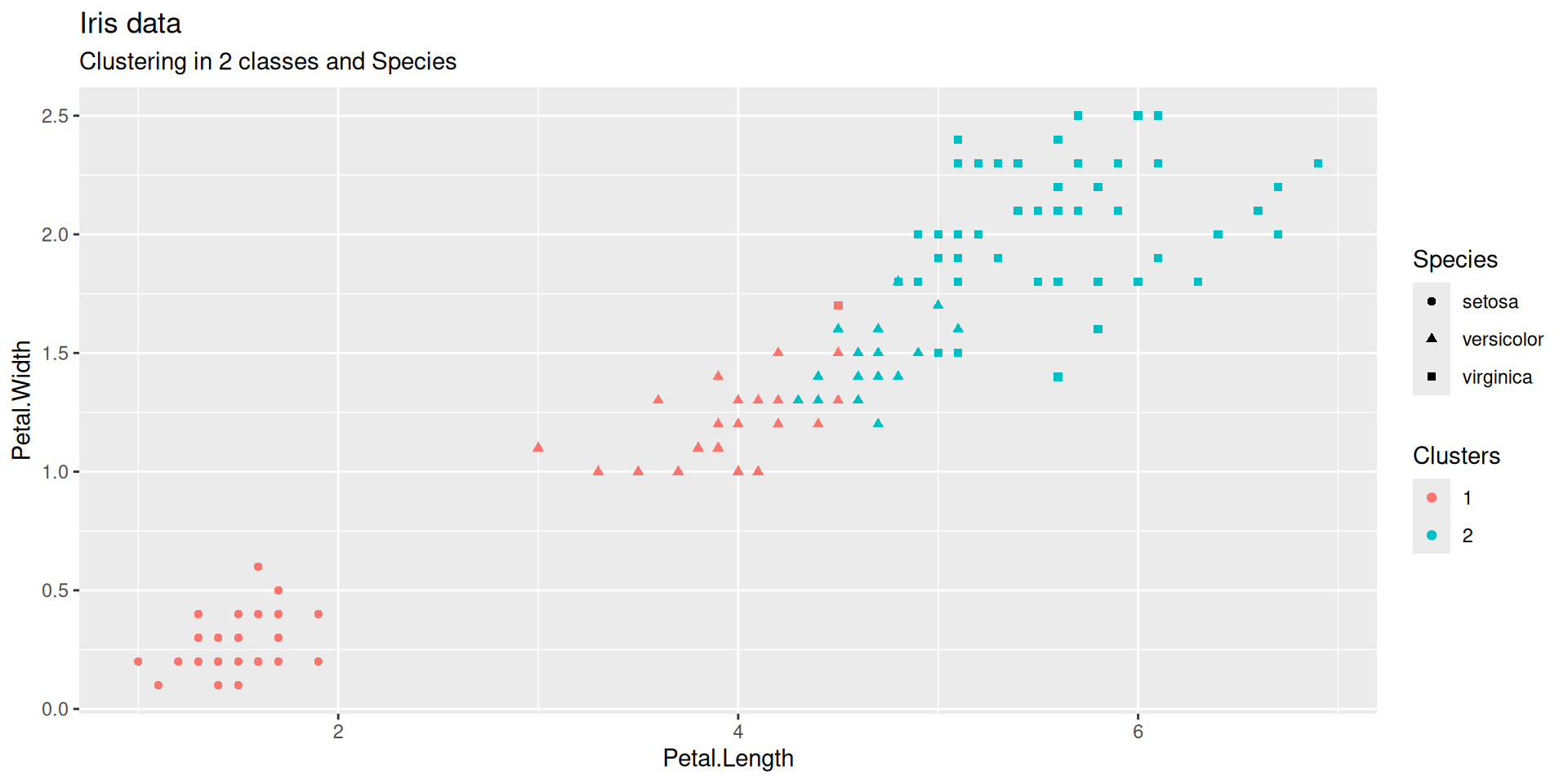
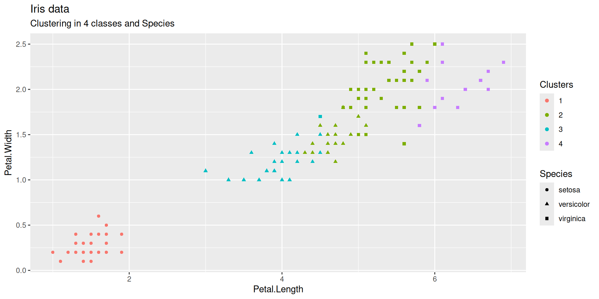
Does the flat clustering obtained by cutting the dendrogram at some height reflect the partition into species?

Cutting a dendrogram: Iris illustration (continued)

Cutting a dendrogram: Iris illustration (continued)

Cutting a dendrogram: Iris illustration (continued)

Cutting a dendrogram: Iris illustration (continued)

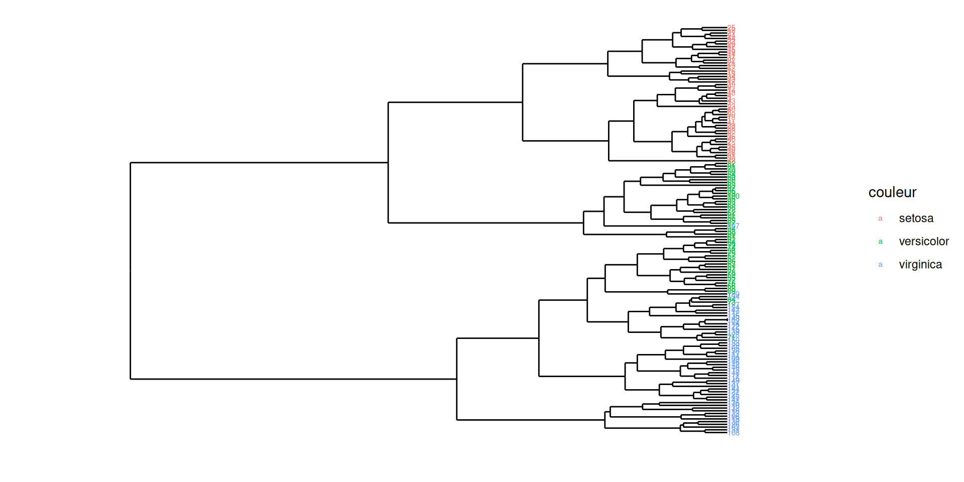
Cutting a dendrogram: better Iris illustration (continued)

The dendextend package offers a set of functions for extending dendrogram objects in , letting you

• visualize and
• compare trees of hierarchical clusterings,

Features:

• Adjust a tree’s graphical parameters - the color, size, type, etc, of its branches, nodes and labels
• Visually and statistically compare different dendrograms to one another

• dendextend

• A dendro gallery

• class of dend

Inside hclust

About class hclust

Results from function hclust() are objects of class hclust :

iris_hclust is an object of class hclust

Function cutree() returns a flat clustering of the dataset

What does height stand for?

What does merge stand for?

What does order stand for?

How different are the different method?

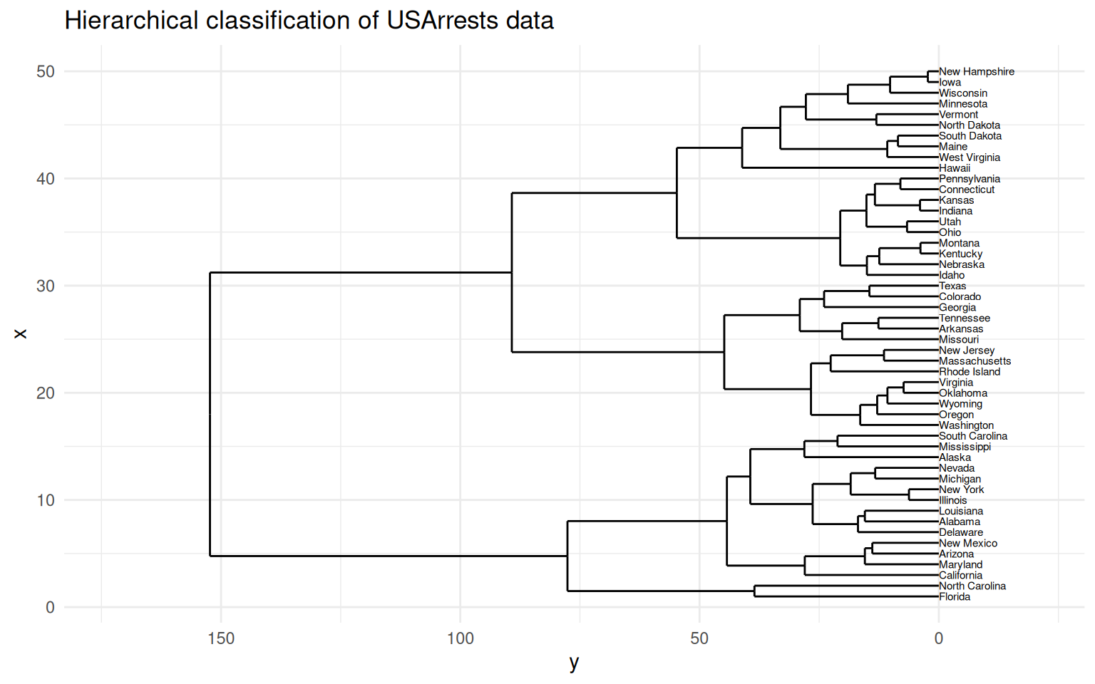
Hierarchical clustering of USArrests

Rows: 50
Columns: 4
$ Murder   <dbl> 13.2, 10.0, 8.1, 8.8, 9.0, 7.9, 3.3, 5.9, 15.4, 17.4, 5.3, 2.…
$ Assault  <int> 236, 263, 294, 190, 276, 204, 110, 238, 335, 211, 46, 120, 24…
$ UrbanPop <int> 58, 48, 80, 50, 91, 78, 77, 72, 80, 60, 83, 54, 83, 65, 57, 6…
$ Rape     <dbl> 21.2, 44.5, 31.0, 19.5, 40.6, 38.7, 11.1, 15.8, 31.9, 25.8, 2…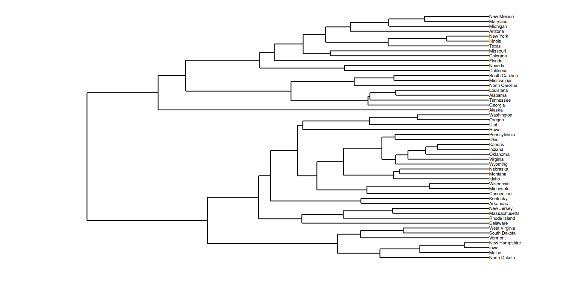

About dendrograms (output dendro_data())

An object of class dendro is a list of 4 objects:

• segments
• labels
• leaf_labels
• class

Questions

• How to build the dendrogram?

• How to choose the cut?

Bird-eye view at hierarchical agglomerative clustering methods

All hierarchical agglomerative clustering methods (HACMs) can be described by the following general algorithm.

1. At each stage distances between clusters are recomputed by the Lance-Williams dissimilarity update formula according to the particular clustering method being used.

2. Identify the 2 closest points and combine them into a cluster (treating existing clusters as points too)

3. If more than one cluster remains, return to step 1.

Greed is good!

• Hierarchical agglomerative clustering methods are examples of greedy algorithms

• Greedy algorithms sometimes compute optimal solutions

  • Huffmann coding (Information Theory)

  • Minimum spanning tree (Graph algorithms)

• Greedy algorithms sometimes compute sub-optimal solutions

  • Set cover (NP-hard problem)

  • …

• Efficient greedy algorithms rely on ad hoc data structures

  • Priority queues

  • Union-Find

Algorithm (detailed)

• Start with \((\mathcal{C}_{i}^{(0)})= (\{ \vec{X}_i \})\) the collection of all singletons.

• At step \(s\), we have \(n-s\) clusters \((\mathcal{C}_{i}^{(s)})\):

  • Find the two most similar clusters according to a criterion \(\Delta\): \[(i,i') = \operatorname{argmin}_{(j,j')} \Delta(\mathcal{C}_{j}^{(s)},\mathcal{C}_{j'}^{(s)})\]

  • Merge \(\mathcal{C}_{i}^{(s)}\) and \(\mathcal{C}_{i'}^{(s)}\) into \(\mathcal{C}_{i}^{(s+1)}\)

  • Keep the \(n-s-2\) other clusters \(\mathcal{C}_{i''}^{(s+1)} = \mathcal{C}_{i''}^{(s)}\)

• Repeat until there is only one cluster left

Analysis

• Complexity: \(O(n^3)\) in general.

• Can be reduced to \(O(n^2)\) (sometimes to \(O(n \log n)\))

  • if the number of possible mergers for a given cluster is bounded.

  • for the most classical distances by maintaining a nearest neighbors list.

Merging criterion based on the distance between points

Minimum linkage:

\[\Delta(\mathcal{C}_i, \mathcal{C}_j) =\min_{\vec{X}_i \in \mathcal{C}_i} \min_{\vec{X}_j \in \mathcal{C}_j} d(\vec{X}_i, \vec{X}_j)\]

Maximum linkage:

\[\Delta(\mathcal{C}_i, \mathcal{C}_j) = \max_{\vec{X}_i \in \mathcal{C}_i} \max_{\vec{X}_j \in \mathcal{C}_j} d(\vec{X}_i, \vec{X}_j)\]

Average linkage:

\[\Delta(\mathcal{C}_i, \mathcal{C}_j) =\frac{1}{|\mathcal{C}_i||\mathcal{C}_j|} \sum_{\vec{X}_i \in \mathcal{C}_i}\sum_{\vec{X}_j \in \mathcal{C}_j} d(\vec{X}_i, \vec{X}_j)\]

Ward’s criterion : minimum variance/inertia criterion

\(\Delta(\mathcal{C}_i, \mathcal{C}_j) = \sum_{\vec{X}_i \in \mathcal{C}_i} \left( d^2(\vec{X}_i, \mu_{\mathcal{C}_i \cup \mathcal{C}_j} ) - d^2(\vec{X}_i, \mu_{\mathcal{C}_i}) \right) +\)

\(\qquad\qquad \qquad \sum_{\vec{X}_j \in \mathcal{C}_j} \left( d^2(\vec{X}_j, \mu_{\mathcal{C}_i \cup \mathcal{C}_j} ) - d^2(\vec{X}_j, \mu_{\mathcal{C}_j}) \right)\)

If \(d\) is the euclidean distance

\[\Delta(\mathcal{C}_i, \mathcal{C}_j) = \frac{ |\mathcal{C}_i||\mathcal{C}_j|}{|\mathcal{C}_i|+ |\mathcal{C}_j|} d^2(\mu_{\mathcal{C}_i}, \mu_{\mathcal{C}_j})\]

Lance-Williams update formulae

Suppose that clusters \(C_{i}\) and \(C_{j}\) were next to be merged

At this point, all of the current pairwise cluster distances are known

The recursive update formula gives the updated cluster distances following the pending merge of clusters \(C_{i}\) and \(C_{j}\)

Let

• \(d_{ij}, d_{ik}\), and \(d_{jk}\) be shortands for the pairwise distances between clusters \(C_{i}, C_{j}\) and \(C_{k}\)

• \(d_{{(ij)k}}\) be shortand for the distance between the new cluster \(C_{i}\cup C_{j}\) and \(C_{k}\) ( \(k\not\in \{i,j\}\) )

Lance-Williams update formulae (continued)

An algorithm belongs to the Lance-Williams family if the updated cluster distance \(d_{{(ij)k}}\) can be computed recursively by

\[d_{(ij)k} = \alpha _{i}d_{ik}+ \alpha _{j}d_{jk}+ \beta d_{ij}+ \gamma |d_{ik}-d_{jk}|\]

where \(\alpha_{i},\alpha _{j},\beta\) , and \(\gamma\) are parameters, which may depend on cluster sizes, that together with the cluster distance function \(d_{ij}\) determine the clustering algorithm.

Clustering algorithms such as

• single linkage,
• complete linkage, and
• group average

method have a recursive formula of the above type

Lance-Williams update formula for Ward’s criterion

\[\begin{array}{rl}d\left(C_i \cup C_j, C_k\right) & = \frac{n_i+n_k}{n_i+n_j+n_k}d\left(C_i, C_k\right) +\frac{n_j+n_k}{n_i+n_j+n_k}d\left(C_j, C_k\right) \\ & \phantom{==}- \frac{n_k}{n_i+n_j+n_k} d\left(C_i, C_j\right)\end{array}\]

\[\alpha_i = \frac{n_i+n_k}{n_i+n_j+n_k} \qquad \alpha_j = \frac{n_j+n_k}{n_i+n_j+n_k}\qquad \beta = \frac{- n_k}{n_i+n_j+n_k}\]

An unfair quotation

Ward’s minimum variance criterion minimizes the total within-cluster variance .fr[Wikipedia]

• Is that correct?

• If corrected, what does it mean?

If we understand the statement as:

for any \(k\), the flat clustering obtained by cutting the dendrogram so as to obtain a \(k\)-clusters partition minimizes the total within-cluster variance/inertia amongst all \(k\)-clusterings

then, the statement is not proved. If it were proved, it would imply \(\mathsf{P}=\mathsf{NP}\)

The total within-cluster variance/inertia is the objective function in the \(k\)-means problem.

The statement is misleading

What happens in Ward’s method?

At each step find the pair of clusters that leads to minimum increase in total within-cluster variance after merging .fr[Wikipedia]

This increase is a weighted squared distance between cluster centers .fr[Wikipedia]

At the initial step, all clusters are singletons (clusters containing a single point). To apply a recursive algorithm under this objective function, the initial distance between individual objects must be (proportional to) squared Euclidean distance.

Views on Inertia:

\[I = \frac{1}{n} \sum_{i=1}^n \|\vec{X}_i - \vec{m} \|^2\]

where \(\vec{m} = \sum_{i=1}^n \frac{1}{n}\vec{X}_i\)

\[I = \frac{1}{2n^2} \sum_{i,j} \|\vec{X}_i - \vec{X}_j\|^2\]

Twice the mean squared distance to the mean equals the mean squared distance between sample points

Recall that for a real random variable \(Z\) with mean \(\mu\)

\[\operatorname{var}(Z) = \mathbb{E}(Z -m)^2 = \inf_a \mathbb{E}(Z -a)^2\]

and

\[\operatorname{var}(Z) = \frac{1}{2} \mathbb{E}(Z -Z')^2\]

where \(Z'\) is an independent copy of \(Z\)

The different formulae for inertia is just mirroring the different views at variance

The inertia is the trace of an empirical covariance matrix.

Decompositions of inertia (Huyghens formula)

• Sample \(x_1,\ldots, x_{n+m}\) with mean \(\bar{X}_{n+m}\) and variance \(V\)

• Partition \(\{1,\ldots,n+m\} = A \cup B\) with \(|A|=n, |B|=m\), \(A \cap B =\emptyset\)

• Let \(\bar{X}_n = \frac{1}{n}\sum_{i \in A} X_i\) and \(\bar{X}_m=\frac{1}{m}\sum_{i \in B}X_i\) \[\bar{X}_{n+m} = \frac{n}{n+m} \bar{X}_{n} +\frac{m}{n+m} \bar{X}_{m}\]

• Let \(V_A\) be the variance of \((x_i)_{i\in A}\), \(V_B\) be the variance of \((x_i)_{i\in B}\)

Decompositions of inertia (Huyghens formula)

• Let \(V_{\text{between}}\) be the variance of a ghost sample with \(n\) copies of \(\bar{X}_n\) and \(m\) copies of \(\bar{X}_m\) \[V_{\text{between}} = \frac{n}{n+m} (\bar{X}_n -\bar{X}_{n+m})^2 + \frac{m}{n+m} (\bar{X}_m -\bar{X}_{n+m})^2\]

• Let \(V_{\text{within}}\) be the weighted mean of variances within classes \(A\) and \(B\) \[V_{\text{within}} = \frac{n}{n+m} V_A + \frac{m}{n+m} V_B\]

Decompositions of inertia

Proposition: Huyghens formula I

\[V = V_{\text{within}} + V_{\text{between}}\]

Huyghens formula can be extended to any number of classes

Proposition: Huyghens (II)

• Sample \(\vec{x}_1, \ldots,\vec{x}_n\) from \(\mathbb{R}^p\) with mean \(\bar{X}_n\), inertia \(I\).

• Let \(A_1, A_2\ldots, A_k\) be a partition of \(\{1,\ldots,n\}\).

• Let \(I_\ell\) (resp. \(\bar{X}^\ell\)) be the inertia (resp. the mean) of sub-sample \(\vec{x}_i, i\in A_\ell\)

• Let \(I_{\text{between}}\) be the inertia of the ghost sample, formed by \(|A_1|\) copies of \(\bar{X}^1\), \(|A_2|\) copies of \(\bar{X}^2\), … \(|A_k|\) copies of \(\bar{X}^k\)

• Let \(I_{\text{within}} = \sum_{\ell=1}^k \frac{|A_\ell|}{n} I_\ell\)

\[I = I_{\text{within}} + I_{\text{between}}\]

Comparing dendrograms

Cophenetic disimilarity

Given a dendrogram, the cophenetic disimilarity between two sample points \(x, x'\) is the intergroup disimilarity at which observations \(x\) and \(x'\) are first joined.

Proposition

A cophenetic disimilarity has the ultrametric property

All triangles are isoceles and the unequal length should be no longer than the length of the two equal sides

Cophenetic correlation coefficient

The cophenetic correlation coefficient measures how faithfully a dendrogram preserves the pairwise distances between the original unmodeled data points

wikipedia]

Computing cophenetic correlation coefficient

In use the dendextend package

single	complete	average	mcquitty	ward.D	centroid	median	ward.D2
0.86	0.73	0.88	0.87	0.86	0.87	0.86	0.87

How to apply general algorithm?

• Lance-Williams dissimilarity update formula calculates dissimilarities between a new cluster and existing points, based on the dissimilarities prior to forming the new cluster

• This formula has 3 parameters

• Each HACM is characterized by its own set of Lance-Williams parameters

Implementations of the general algorithm

Stored matrix approach

Use matrix, and then apply Lance-Williams to recalculate dissimilarities between cluster centers. Storage \(O(N^2)\) and time at least \(O(N^2)\), but is \(\Theta(N^3)\) if matrix is scanned linearly

Stored data approach

\(O(N)\) space for data but recompute pairwise dissimilarities, needs \(\Theta(N^3)\) time

Sorted matrix approach

\(O(N^2)\) to calculate dissimilarity matrix, \(O(N^2 \log N)\) to sort it, \(O(N^2)\) to construct hierarchy, but one need not store the data set, and the matrix can be processed linearly, which reduces disk accesses

Agglomerative Clustering Heuristic

• Start with very small clusters (a sample point by cluster?)

• Merge iteratively the most similar clusters according to some greedy criterion \(\Delta\).

• Generates a hierarchy of clusterings instead of a single one.

• Need to select the number of cluster afterwards.

• Several choice for the merging criterion

• Examples:

  • Minimum Linkage: merge the closest cluster in term of the usual distance

  • Ward’s criterion: merge the two clusters yielding the less inner inertia loss (minimum variance criterion)

Packages

• • ggdendro
  • dendextend
  • dendroextras
• • scipy
  • scikit-learn

The End

Hierarchical Clustering