Tables manipulation with dplyr

Analyse de Données Master MIDS

Équipe EAD

LPSM Université Paris-Cité

2021-12-21

Tables

Tables (examples)

Speadsheets (Excel)
Relational tables
Dataframes in datascience frameworks
- : data.frame, tibble, …
- : pandas.dataframe
- spark: dataframe
- Dask: dataframe
- and many others

Tables (Why ?)

In Data Science, each framework comes with its own flavor(s) of table(s)

Tables from relational databases serve as inspiration

In legacy dataframes shape the life of statisticians and data scientists

The purpose of this session is

describe dataframes from an end-user viewpoint (we leave aside implementations)
presenting tools for
- accessing information within dataframes (querying)
- summarizing information (aggregation queries)
- cleaning/cleaning dataframes (tidying)

Loading tables and packages

require("tidyverse")      # All we need is there
require("nycflights13")    # for flight data
require("gt")
require("kableExtra")
# 
data(flights)

About loaded packages

Metapackage tidyverse provides tools to create, query, tidy dataframes as well as tools to load data from various sources and save them in persistent storage
nycflights13 provides the dataframes we play with
gt for tayloring table displays

The `flights` table

head(flights) |>
  glimpse(width = 30)

Rows: 6
Columns: 19
$ year           <int> 2013,…
$ month          <int> 1, 1,…
$ day            <int> 1, 1,…
$ dep_time       <int> 517, …
$ sched_dep_time <int> 515, …
$ dep_delay      <dbl> 2, 4,…
$ arr_time       <int> 830, …
$ sched_arr_time <int> 819, …
$ arr_delay      <dbl> 11, 2…
$ carrier        <chr> "UA",…
$ flight         <int> 1545,…
$ tailnum        <chr> "N142…
$ origin         <chr> "EWR"…
$ dest           <chr> "IAH"…
$ air_time       <dbl> 227, …
$ distance       <dbl> 1400,…
$ hour           <dbl> 5, 5,…
$ minute         <dbl> 15, 2…
$ time_hour      <dttm> 2013…

A dataframe is a two-ways (two-dimensional) table
head(df) displays the first 6 rows of its first argument
The vectors making a dataframe may have different types/classes (a dataframe is not a matrix)
Compare str(), glimpse(), head()

Table schema

A table is a list of columns

Each column has

name and
type (class in

glimpse(flights,   #<<
        width=50)

Rows: 336,776
Columns: 19
$ year           <int> 2013, 2013, 2013, 2013, 2…
$ month          <int> 1, 1, 1, 1, 1, 1, 1, 1, 1…
$ day            <int> 1, 1, 1, 1, 1, 1, 1, 1, 1…
$ dep_time       <int> 517, 533, 542, 544, 554, …
$ sched_dep_time <int> 515, 529, 540, 545, 600, …
$ dep_delay      <dbl> 2, 4, 2, -1, -6, -4, -5, …
$ arr_time       <int> 830, 850, 923, 1004, 812,…
$ sched_arr_time <int> 819, 830, 850, 1022, 837,…
$ arr_delay      <dbl> 11, 20, 33, -18, -25, 12,…
$ carrier        <chr> "UA", "UA", "AA", "B6", "…
$ flight         <int> 1545, 1714, 1141, 725, 46…
$ tailnum        <chr> "N14228", "N24211", "N619…
$ origin         <chr> "EWR", "LGA", "JFK", "JFK…
$ dest           <chr> "IAH", "IAH", "MIA", "BQN…
$ air_time       <dbl> 227, 227, 160, 183, 116, …
$ distance       <dbl> 1400, 1416, 1089, 1576, 7…
$ hour           <dbl> 5, 5, 5, 5, 6, 5, 6, 6, 6…
$ minute         <dbl> 15, 29, 40, 45, 0, 58, 0,…
$ time_hour      <dttm> 2013-01-01 05:00:00, 201…

flights has 19 columns
Each column is a sequence (vector) of items with the same type/class
All columns have the same length
flights has 336776 rows
In parlance, a row is (often) called a tuple
In parlance, a column is (often) called a variable

Column types

class	columns
`integer`	‘year’ ‘month’ ‘day’ ‘dep_time’ ‘sched_dep_time’ ‘arr_time’ ‘sched_arr_time’ ‘flight’
`numeric`	‘dep_delay’ ‘arr_delay’ ‘air_time’ ‘distance’ ‘hour’ ‘minute’
`character`	‘carrier’ ‘tailnum’ ‘origin’ ‘dest’
`POSIXct`	‘time_hour’
`POSIXt`	‘time_hour’

A column, as a vector, may be belong to different classes

Other classes: factor for categorical variables

Columns dest, origin carrier could be coerced as factors

Should columns dest and origin be coerced to the same factor?

`nycflights13`

Columns specification

as.col_spec(flights)

cols(
  year = col_integer(),
  month = col_integer(),
  day = col_integer(),
  dep_time = col_integer(),
  sched_dep_time = col_integer(),
  dep_delay = col_double(),
  arr_time = col_integer(),
  sched_arr_time = col_integer(),
  arr_delay = col_double(),
  carrier = col_character(),
  flight = col_integer(),
  tailnum = col_character(),
  origin = col_character(),
  dest = col_character(),
  air_time = col_double(),
  distance = col_double(),
  hour = col_double(),
  minute = col_double(),
  time_hour = col_datetime(format = "")
)

$\approx$ table schema in relational databases

Column specifications are useful when loading dataframes from structured text files like .csv files

.csv files do not contain typing information

File loaders from package readr can be tipped about column classes using column specifications

SQL and Relational algebra with `dplyr`

SQL stands for structured/simple Query Language
A query language elaborated during the 1970’s at IBM by E. Codd
Geared towards exploitation of collections of relational tables
Less powerful but simpler to use than a programming language
dplyr is a principled -friendly implementation of SQL ideas (and other things)

At the core of SQL lies the idea of a table calculus called relational algebra

Relational algebra (basics)

Convention: $R$ is a table with columns $A_1, \ldots, A_k$

Projection (picking columns)

$\pi(R, A_1, A_3)$

Selection/Filtering (picking rows)

$\sigma(R, {\text{condition}})$

Join (mulitple tables operation)

$\bowtie(R,S, {\text{condition}})$

Any operation produces a table

The schema of the derived table depends on the operation (but does not depend on the content/value of the operands)

Table calculus relies on a small set of basic operations $\pi, \sigma, \bowtie$

Each operation has one or two table operands and produce a table

There is more to SQL than relational algebra

Projection $\pi$

$\pi(R, {A_1, A_3})$

A projection $\pi(\cdot, {A_1, A_3})$ is defined by a set of column names, say $A_1, A_3$

If $R$ has columns with given names, the result is a table with names $A_1, A_3$ and one row per row of $R$

A projection is parametrized by a list of column names

Package `dplyr`

https://dplyr.tidyverse.org

Base provides tools to perform relational algebra operations

But:

Base does not provide a consistent API
The lack of a consistent API makes operation chaining tricky

`dplyr` verbs

Five basic verbs:

Pick observations/rows by their values (filter()) σ(…)
Pick variables by their names (select()) π(…)
Reorder the rows (arrange())
Create new variables with functions of existing variables (mutate())
Collapse many values down to a single summary (summarise())

And

group_by() changes the scope of each function from operating on the entire dataset to operating on it group-by-group

tidyverse

All verbs work similarly:

The first argument is a data frame (table).

The subsequent arguments describe what to do with the data frame, using the variable/column names (without quotes)

The result is a new data frame (table)

`dplyr::select()` as a projection operator (π)

$\pi(R, \underbrace{A_1, \ldots, A_3}_{\text{column names}})$

select(R, A1, A3) #<<

or, equivalently

R |> select(A1, A3) #<<

|> is the pipe operator

x |> f(y, z) is translated to f(x, y, z) and then evaluated

`dplyr::select()`

Function select has a variable number of arguments
Function select has a variable number of arguments
Function select allows to pick column by names (and much more)
Note that in the current environment, there are no objects called A1, A3
The consistent API allows to use the pipe operator

Caution

There is also a select() function in base R

Toy tables

spam <- set.seed(42)

R <-  tibble(A1=seq(2, 10, 2),
             A2=sample(letters, 5),
             A3=seq(from=date("2021-10-21"),
                    to=date("2021-11-20"),
                    by=7),
             D=sample(letters, 5))

S <- tibble(E=c(3,4,6,9, 10),
            F=sample(letters, 5),
            G=seq(from=date("2021-10-21"),
                   to=date("2021-10-21")+4, by=1),
            D=sample(letters,5)
          )

R
A1	A2	A3	D
2	q	2021-10-21	r
4	e	2021-10-28	q
6	a	2021-11-04	o
8	j	2021-11-11	g
10	d	2021-11-18	d

S
E	F	G	D
3	y	2021-10-21	o
4	e	2021-10-22	c
6	n	2021-10-23	i
9	t	2021-10-24	d
10	r	2021-10-25	e

Projecting toy tables

R |> 
  dplyr::select(A2,D) |> 
  knitr::kable(caption="Projecting R")

Projecting R
A2	D
q	r
e	q
a	o
j	g
d	d

R |> 
  dplyr::select(- where(is.character)) |> 
  knitr::kable(caption="Projecting R, all but character columns")

Projecting R, all but character columns
A1	A3
2	2021-10-21
4	2021-10-28
6	2021-11-04
8	2021-11-11
10	2021-11-18

Projecting `flights` on `origin` and `dest`

flights |>
  select(origin, dest) |>  #<<
  head()

# A tibble: 6 × 2
  origin dest 
  <chr>  <chr>
1 EWR    IAH  
2 LGA    IAH  
3 JFK    MIA  
4 JFK    BQN  
5 LGA    ATL  
6 EWR    ORD

A more readable equivalent of

head(select(flights, origin, dest), 10)

SELECT 
  origin, dest
FROM 
  flights
LIMIT 6;

$\sigma(R, \text{condition})$

A selection/filtering operation is defined by a condition that can be checked on the rows of tables with convenient schema
$\sigma(R, \text{condition})$ returns a table with the same schema as $R$
The resulting table contains the rows/tuples of $R$ that satisfy $\text{condition}$
$\sigma(R, \text{FALSE})$ returns an empty table with the same schema as $R$

Chaining filtering and projecting

start <- date("2021-10-27")
end <- start + 21

R |>
#  filter(A2 > "n") |>  #<<
  filter(between(A3, start, end)) |>
  select(A1, A3) #<<

# A tibble: 3 × 2
     A1 A3        
  <dbl> <date>    
1     4 2021-10-28
2     6 2021-11-04
3     8 2021-11-11

Selecting `flights` based on `origin` and `dest`

and then projecting on dest, time_hour, carrier

flights |>
  filter(dest %in% c('ATL', 'LAX'), #<<
         origin == 'JFK') |>
  select(dest, time_hour, carrier) |> #<<
  head()

# A tibble: 6 × 3
  dest  time_hour           carrier
  <chr> <dttm>              <chr>  
1 LAX   2013-01-01 06:00:00 UA     
2 ATL   2013-01-01 06:00:00 DL     
3 LAX   2013-01-01 07:00:00 VX     
4 LAX   2013-01-01 07:00:00 B6     
5 LAX   2013-01-01 07:00:00 AA     
6 ATL   2013-01-01 08:00:00 DL

In SQL ( parlance:

SELECT 
  dest, time_hour, carrier
FROM 
  flights
WHERE 
  dest IN ('ATL', 'LAX') AND
  origin = 'JFK'
LIMIT 6

Logical operations

filter(R, condition_1, condition_2) is meant to return the rows of R that satisfy condition_1 and condition_2
filter(R, condition_1 & condition_2) is an equivalent formulation
filter(R, condition_1 | condition_2) is meant to return the rows of R that satisfy condition_1 or condition_2 (possibly both)
filter(R, xor(condition_1,condition_2)) is meant to return the rows of R that satisfy either condition_1 or condition_2 (just one of them)
filter(R, ! condition_1) is meant to return the rows of R that do not satisfy condition_1

Missing values!

Numerical column dep_time contains many NA's (missing values)

# flights |> pull(dep_time) |> summary()
summary(flights$dep_time)

   Min. 1st Qu.  Median    Mean 3rd Qu.    Max.    NA's 
      1     907    1401    1349    1744    2400    8255

Missing values (NA and variants) should be handled with care

NA & TRUE

[1] NA

NA | TRUE

[1] TRUE

Truth tables for three-valued logic

uses three-valued logic

Generate complete truth tables for and, or, xor

v <- c(TRUE, FALSE, NA) # truth values

list_tt <- map(c(`&`, `|`, xor),  #<<
               ~ outer(v, v, .x)) #<<

for (i in seq_along(list_tt)){
  colnames(list_tt[[i]]) <- v
  rownames(list_tt[[i]]) <- v
}

names(list_tt) <- c('& AND',
                    'OR',
                    'XOR')

& AND
	TRUE	FALSE	NA
TRUE	TRUE	FALSE	NA
FALSE	FALSE	FALSE	FALSE
NA	NA	FALSE	NA

OR
	TRUE	FALSE	NA
TRUE	TRUE	TRUE	TRUE
FALSE	TRUE	FALSE	NA
NA	TRUE	NA	NA

XOR
	TRUE	FALSE	NA
TRUE	FALSE	TRUE	NA
FALSE	TRUE	FALSE	NA
NA	NA	NA	NA

`slice()`: choosing rows based on location

In base dataframe cells can be addressed by indices

flights[5000:5010,seq(1, 19, by=5)] returns rows 5000:5010 and columns 1, 6, 11 from dataframe flights

This can be done in a (verbose) dplyr way using slice() and select()

flights |>
  slice(5001:5005) |>  #<<
  select(seq(1, 19, by=5))

# A tibble: 5 × 4
   year dep_delay flight distance
  <int>     <dbl>  <int>    <dbl>
1  2013         3   4437      602
2  2013        43   1016      187
3  2013        -2   2190     1089
4  2013        -1     91     2576
5  2013         5   2131      502

combined with aggregation (group_by()) variants of slice_ may be used to perform windowing operations

Useful variant slice_sample()

Joins : multi-table queries

Note

$\bowtie(R,S, {\text{condition}})$

stands for

join rows/tuples of $R$ and rows/tuples of $S$ that satisfy $\text{condition}$

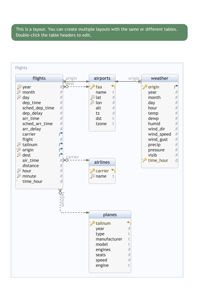
`nycflights` tables

The nycflights13 package offers five related tables:

Fact tables:
- flights
- weather (hourly weather conditions at different locations)
Dimension tables:
- airports (airports full names, location, …)
- planes (model, manufacturer, year, …)
- airlines (full names)

This is an instance of a Star Schema

About Star schemas

Fact tables record measurements for a specific event
Fact tables generally consist of numeric values, and foreign keys to dimensional data where descriptive information is kept
Dimension tables record informations about entities involved in events recorded in Fact tables

weather conditions

weather |>
  glimpse(width = 50)

Rows: 26,115
Columns: 15
$ origin     <chr> "EWR", "EWR", "EWR", "EWR", "…
$ year       <int> 2013, 2013, 2013, 2013, 2013,…
$ month      <int> 1, 1, 1, 1, 1, 1, 1, 1, 1, 1,…
$ day        <int> 1, 1, 1, 1, 1, 1, 1, 1, 1, 1,…
$ hour       <int> 1, 2, 3, 4, 5, 6, 7, 8, 9, 10…
$ temp       <dbl> 39.02, 39.02, 39.02, 39.92, 3…
$ dewp       <dbl> 26.06, 26.96, 28.04, 28.04, 2…
$ humid      <dbl> 59.37, 61.63, 64.43, 62.21, 6…
$ wind_dir   <dbl> 270, 250, 240, 250, 260, 240,…
$ wind_speed <dbl> 10.35702, 8.05546, 11.50780, …
$ wind_gust  <dbl> NA, NA, NA, NA, NA, NA, NA, N…
$ precip     <dbl> 0, 0, 0, 0, 0, 0, 0, 0, 0, 0,…
$ pressure   <dbl> 1012.0, 1012.3, 1012.5, 1012.…
$ visib      <dbl> 10, 10, 10, 10, 10, 10, 10, 1…
$ time_hour  <dttm> 2013-01-01 01:00:00, 2013-01…

Connecting `flights` and `weather`

We want to complement information in flights using data weather

Motivation: we would like to relate delays (arr_delay) and weather conditions

can we explain (justify) delays using weather data?
can we predict delays using weather data?

⋈

For each flight (row in flights)

year, month, day, hour (computed from time_hour) indicate the approaximate time of departure
origin indicates the airport where the plane takes off

Each row of weather contains corresponding information

for each row of flights we look for rows of weather with matching values in year, month, day, hour and origin

NATURAL INNER JOIN between the tables

`inner_join`: natural join

f_w <- flights |>
  inner_join(weather) #<<

f_w |> 
  select(seq(1, 
             ncol(f_w),
             by=2)) |> 
  glimpse(width=50)

Rows: 335,220
Columns: 14
$ year           <int> 2013, 2013, 2013, 2013, 2…
$ day            <int> 1, 1, 1, 1, 1, 1, 1, 1, 1…
$ sched_dep_time <int> 515, 529, 540, 545, 600, …
$ arr_time       <int> 830, 850, 923, 1004, 812,…
$ arr_delay      <dbl> 11, 20, 33, -18, -25, 12,…
$ flight         <int> 1545, 1714, 1141, 725, 46…
$ origin         <chr> "EWR", "LGA", "JFK", "JFK…
$ air_time       <dbl> 227, 227, 160, 183, 116, …
$ hour           <dbl> 5, 5, 5, 5, 6, 5, 6, 6, 6…
$ time_hour      <dttm> 2013-01-01 05:00:00, 201…
$ dewp           <dbl> 28.04, 24.98, 26.96, 26.9…
$ wind_dir       <dbl> 260, 250, 260, 260, 260, …
$ wind_gust      <dbl> NA, 21.86482, NA, NA, 23.…
$ pressure       <dbl> 1011.9, 1011.4, 1012.1, 1…

Join schema

Rows: 335,220
Columns: 28
$ year           <int> 2013, 2013, 2013, 2013, 2…
$ month          <int> 1, 1, 1, 1, 1, 1, 1, 1, 1…
$ day            <int> 1, 1, 1, 1, 1, 1, 1, 1, 1…
$ dep_time       <int> 517, 533, 542, 544, 554, …
$ sched_dep_time <int> 515, 529, 540, 545, 600, …
$ dep_delay      <dbl> 2, 4, 2, -1, -6, -4, -5, …
$ arr_time       <int> 830, 850, 923, 1004, 812,…
$ sched_arr_time <int> 819, 830, 850, 1022, 837,…
$ arr_delay      <dbl> 11, 20, 33, -18, -25, 12,…
$ carrier        <chr> "UA", "UA", "AA", "B6", "…
$ flight         <int> 1545, 1714, 1141, 725, 46…
$ tailnum        <chr> "N14228", "N24211", "N619…
$ origin         <chr> "EWR", "LGA", "JFK", "JFK…
$ dest           <chr> "IAH", "IAH", "MIA", "BQN…
$ air_time       <dbl> 227, 227, 160, 183, 116, …
$ distance       <dbl> 1400, 1416, 1089, 1576, 7…
$ hour           <dbl> 5, 5, 5, 5, 6, 5, 6, 6, 6…
$ minute         <dbl> 15, 29, 40, 45, 0, 58, 0,…
$ time_hour      <dttm> 2013-01-01 05:00:00, 201…
$ temp           <dbl> 39.02, 39.92, 39.02, 39.0…
$ dewp           <dbl> 28.04, 24.98, 26.96, 26.9…
$ humid          <dbl> 64.43, 54.81, 61.63, 61.6…
$ wind_dir       <dbl> 260, 250, 260, 260, 260, …
$ wind_speed     <dbl> 12.65858, 14.96014, 14.96…
$ wind_gust      <dbl> NA, 21.86482, NA, NA, 23.…
$ precip         <dbl> 0, 0, 0, 0, 0, 0, 0, 0, 0…
$ pressure       <dbl> 1011.9, 1011.4, 1012.1, 1…
$ visib          <dbl> 10, 10, 10, 10, 10, 10, 1…

The schema of the result is the union of the schemas of the operands

A tuple from flights matches a tuple from weather if the tuple have the same values in the common columns:

 [1] "year"           "month"          "day"            "dep_time"      
 [5] "sched_dep_time" "dep_delay"      "arr_time"       "sched_arr_time"
 [9] "arr_delay"      "carrier"        "flight"         "tailnum"       
[13] "origin"         "dest"           "air_time"       "distance"      
[17] "hour"           "minute"         "time_hour"      "temp"          
[21] "dewp"           "humid"          "wind_dir"       "wind_speed"    
[25] "wind_gust"      "precip"         "pressure"       "visib"

Which columns are used when joining tables $R$ and $S$?

default behavior of inner_join: all columns shared by $R$ and $S$. Common columns have the same name in both schema. They are expected to have the same class
manual definition: in many settings, we want to overrule the default behavior. We specify manually which column from $R$ should match which column from $S$

Natural join of `flights` and `weather`:

common_names <- base::intersect(names(weather),
                                names(flights))

setequal(
  inner_join(flights, weather),
  inner_join(flights,
             weather,
             by=common_names)
)

[1] TRUE

Are you surprised by the next chunk?

dtu  <- inner_join(flights,
           weather,
           by=c("year", "month", "day", "origin", "hour"))

dtv <- inner_join(flights,
           weather,
           by=c("origin", "time_hour"))

# setequal(dtu, dtv)

Recall that columns year, month day hour can be computed from time_hour

flights |>
  filter(year!=year(time_hour) |
         month!=month(time_hour) |
         day!=day(time_hour) |
         hour!=hour(time_hour)) |>
  nrow()

[1] 0

The two results do not have the same schema!

setdiff(colnames(dtv), colnames(dtu))

[1] "year.x"    "month.x"   "day.x"     "hour.x"    "time_hour" "year.y"   
[7] "month.y"   "day.y"     "hour.y"

setdiff(colnames(dtu), colnames(dtv))

[1] "year"        "month"       "day"         "hour"        "time_hour.x"
[6] "time_hour.y"

Fixing

dtu  <- inner_join(flights,
           weather,
           by=c("year", "month", "day", "origin", "hour"),
           suffix= c("", ".y")) |>  #<<
           select(-ends_with(".y"))  #<<

dtv <- inner_join(flights,
           weather,
           by=c("origin", "time_hour"),
           suffix= c("", ".y")) |>  #<<
           select(-ends_with(".y"))  #<<

setequal(dtu, dtv)

[1] TRUE

About `inner_join`

inner_join(
  x, y,
  by = NULL,      #<<
  copy = FALSE,
  suffix = c(".x", ".y"), #<<
  ...,
  keep = FALSE,  #<<
  na_matches = "na")  #<<

by:
- by=c("A1", "A3", "A7") row r from R and s from S match if r.A1 == s.A1, r.A3 == s.A3, r.A7 == s.A7
- by=c("A1"="B", "A3"="C", "A7"="D") row r from R and s from S match if r.A1 == s.B, r.A3 == s.C, r.A7 == s.D
suffix: If there are non-joined duplicate variables in x and y, these suffixes will be added to the output to disambiguate them.
keep: Should the join keys from both x and y be preserved in the output?
na_matches: Should NA and NaN values match one another?

Join flavors

Different flavors of join can be used to join one table to columns from another, matching values with the rows that they correspond to

Each join retains a different combination of values from the tables

left_join(x, y, by = NULL, suffix = c(".x", ".y"), ...) Join matching values from y to x. Retain all rows of x padding missing values from y by NA
semi_join …
anti_join …

Toy examples : `inner_join`

R
A1	A2	A3	D
2	q	2021-10-21	r
4	e	2021-10-28	q
6	a	2021-11-04	o
8	j	2021-11-11	g
10	d	2021-11-18	d

S
E	F	G	D
3	y	2021-10-21	o
4	e	2021-10-22	c
6	n	2021-10-23	i
9	t	2021-10-24	d
10	r	2021-10-25	e

inner_join(S, R, by=c(“E”=“A1”))
E	F	G	D.x	A2	A3	D.y
4	e	2021-10-22	c	e	2021-10-28	q
6	n	2021-10-23	i	a	2021-11-04	o
10	r	2021-10-25	e	d	2021-11-18	d

Toy examples : `left_join`

R
A1	A2	A3	D
2	q	2021-10-21	r
4	e	2021-10-28	q
6	a	2021-11-04	o
8	j	2021-11-11	g
10	d	2021-11-18	d

S
E	F	G	D
3	y	2021-10-21	o
4	e	2021-10-22	c
6	n	2021-10-23	i
9	t	2021-10-24	d
10	r	2021-10-25	e

left_join(S, R, by=c(“E”=“A1”))
E	F	G	D.x	A2	A3	D.y
3	y	2021-10-21	o	NA	NA	NA
4	e	2021-10-22	c	e	2021-10-28	q
6	n	2021-10-23	i	a	2021-11-04	o
9	t	2021-10-24	d	NA	NA	NA
10	r	2021-10-25	e	d	2021-11-18	d

Toy examples : `semi_join` `anti_join`

R
A1	A2	A3	D
2	q	2021-10-21	r
4	e	2021-10-28	q
6	a	2021-11-04	o
8	j	2021-11-11	g
10	d	2021-11-18	d

S
E	F	G	D
3	y	2021-10-21	o
4	e	2021-10-22	c
6	n	2021-10-23	i
9	t	2021-10-24	d
10	r	2021-10-25	e

semi_join(S, R, by=c(“E”=“A1”))
E	F	G	D
4	e	2021-10-22	c
6	n	2021-10-23	i
10	r	2021-10-25	e

anti_join(S, R, by=c(“E”=“A1”))
E	F	G	D
3	y	2021-10-21	o
9	t	2021-10-24	d

Conditional/ $\theta$ -join

In relational databases, joins are not restricted to natural joins

\[U \leftarrow R \bowtie_{\theta} S\]

reads as

\[\begin{array}{rl} T & \leftarrow R \times S\\ U & \leftarrow \sigma(T, \theta)\end{array}\]

where

$R \times S$ is the cartesian product of $R$ and $S$
$\theta$ is a boolean expression that can be evaluated on any tuple of $R \times S$

Do we need conditional/ $\theta$ -joins?

Note

: We can implement $\theta$/conditional-joins by pipelining a cross product and a filtering

Caution

: Cross products are costly:

$\#\text{rows}(R \times S) = \#\text{rows}(R) \times \#\text{rows}(S)$
$\#\text{cols}(R \times S) = \#\text{cols}(R) + \#\text{cols}(S)$

Do we need conditional/ $\theta$ -joins?

Note

: RDBMS use query planning and optimization, indexing to circumvent the cross product bottleneck (when possible)

Tip

: if we need to perform a $\theta$-join

outsource it to a RDBMS, or
design an ad hoc pipeline

A conditional join between `flights` and `weather`

The natural join between flights and weather we implemented can be regarded as an ad hoc conditional join between normalized versions of weather and flights
Table flights and weather are redundant: year, month, day, hour can be computed from time_hour
Assume flights and weather are trimmed so as to become irredundant
The conditional join is then based on truncations of variables time_hour

SELECT 
  *
FROM 
  flights AS f, weather AS w
WHERE 
  date_trunc('hour', f.time_hour) = date_trunc('hour', w.time_hour)

Adding redundant columns to flights and weather allows us to transform a tricky conditional join into a simple natural join

Creating new columns

Creation of new columns may happen

on the fly
when altering (enriching) the schema of a table

In databases, creation of new columns may be the result of a query or be the result of altering a table schema with ALTER TABLE ADD COLUMN ...

In tidyverse() we use verbs mutate or add_column to add columns to the input table

`mutate`

mutate(   #<<
  .data,
  new_col= expression, #<<
  ...,   #<<
  .keep = c("all", "used", "unused", "none"),
  .before = NULL,
  .after = NULL
)

.data: the input data frame

new_col= expression:

new_col is the name of a new column
expression is evaluated on each row of .data or it is a vector of length 1
all is the default behavior, retains all columns from .data

Creating a categorical column to spot large delays

breaks_delay <- with(flights,
  c(min(arr_delay, na.rm=TRUE),
    0, 30,
    max(arr_delay, na.rm=TRUE))
)

level_delay <- c("None",
                 "Moderate",
                 "Large")

flights |>
  mutate(large_delay = cut(
    arr_delay,  #<<
    breaks=breaks_delay, #<<
    labels=level_delay,  #<<
    ordered_result=TRUE)) |>   #<<
  select(large_delay, arr_delay) |>
  sample_n(5)

# A tibble: 5 × 2
  large_delay arr_delay
  <ord>           <dbl>
1 Large             219
2 Moderate           18
3 None              -19
4 None              -16
5 None               -1

flights |>
  mutate(foo = if_else(arr_time > sched_arr_time,        #<<
                              arr_time - sched_arr_time,
                              0L,
                              missing = NA_integer_)) |>
  group_by( (foo >0) & abs(foo - arr_delay)  > 100) |>
  summarise(N=n())

# A tibble: 3 × 2
  `(foo > 0) & abs(foo - arr_delay) > 100`      N
  <lgl>                                     <int>
1 FALSE                                    322281
2 TRUE                                       5157
3 NA                                         9338

Changing the class of a column

flights |>
  mutate(large_delay = cut(arr_delay,  #<<
    breaks=breaks_delay,
    labels=level_delay,
    ordered_result=TRUE),
    origin = as.factor(origin), #<<
    dest = as.factor(dest)    #<<
  ) |>
  select(
    large_delay,
    arr_delay,
    origin,
    dest) |>
  sample_n(5)

# A tibble: 5 × 4
  large_delay arr_delay origin dest 
  <ord>           <dbl> <fct>  <fct>
1 None              -44 LGA    CVG  
2 None              -15 EWR    DAY  
3 Large             136 EWR    DEN  
4 None               -9 EWR    TPA  
5 Moderate           14 LGA    TPA

Tidy tables

Tidying tables is part of data cleaning

A (tidy) dataset is a collection of values, usually either numbers (if quantitative) or strings (if qualitative)

Values are organised in two ways

Every value belongs to a variable and an observation

A variable contains all values that measure the same underlying attribute (like height, temperature, duration) across units

An observation contains all values measured on the same unit (like a person, or a day, or a race) across attributes

The principles of tidy data are tied to those of relational databases and Codd’s relational algebra

Codd’s principles

Information is represented logically in tables
Data must be logically accessible by table, primary key, and column.
Null values must be uniformly treated as “missing information,” not as empty strings, blanks, or zeros.
Metadata (data about the database) must be stored in the database just as regular data is
A single language must be able to define data, views, integrity constraints, authorization, transactions, and data manipulation
Views must show the updates of their base tables and vice versa
A single operation must be available to do each of the following operations: retrieve data, insert data, update data, or delete data
Batch and end-user operations are logically separate from physical storage and access methods
Batch and end-user operations can change the database schema without having to recreate it or the applications built upon it
Integrity constraints must be available and stored in the metadata, not in an application program
The data manipulation language of the relational system should not care where or how the physical data is distributed and should not require alteration if the physical data is centralized or distributed
Any row processing done in the system must obey the same integrity rules and constraints that set-processing operations do

dplyr functions expect and return tidy tables

In a tidy table

Each variable is a column
Each observation is a row
Every cell is a single value

In order to tell whether a table is tidy, we need to know what is the population under investigation, what are the observations/individuals, which measures are performed on each individual, …

Untidy data

Column headers are values, not variable names.

Multiple variables are stored in one column.

Variables are stored in both rows and columns.

Multiple types of observational units are stored in the same table.

A single observational unit is stored in multiple tables.

…

Functions from `tidyr::...`

pivot_wider and pivot_longer
separate and unite
Handling missing values with complete, fill, …
…

tidyr website

Pivot longer

pivot_longer() is commonly needed to tidy wild-caught datasets as they often optimise for ease of data entry or ease of comparison rather than ease of analysis.

messy <- tibble::tribble(
  ~row, ~a, ~b, ~c,
  "A", 1, 4, 7,
  "B", 2, 5, 8,
  "C", 3, 6, 9,
)
messy |> kable()

row	a	b	c
A	1	4	7
B	2	5	8
C	3	6	9

messy_long <- messy |> 
  pivot_longer(
    cols=c(-row),  #<<
    names_to = "name",
    values_to = "value")
  
messy_long  |> 
  kable()

row	name	value
A	a	1
A	b	4
A	c	7
B	a	2
B	b	5
B	c	8
C	a	3
C	b	6
C	c	9

Pivot wider

pivot_wider(  #<<
  data,
  id_cols = NULL, #<<
  names_from = name, #<<
  names_prefix = "",
  values_from = value, #<<
  ...
)

some optional arguments are missing

When reporting, we often use pivot_wider (explicitely or implicitely) to make results more readable, possibly to conform to a tradition

Life tables in demography and actuarial science
Longitudinal data
See slide How many flights per day of week per departure airport?

`pivot_wider()` in action

messy_long |>
  pivot_wider( 
  id_cols = c("row"), #<<
  names_from = name, #<<
  names_prefix = "",
  values_from = value
)

# A tibble: 3 × 4
  row       a     b     c
  <chr> <dbl> <dbl> <dbl>
1 A         1     4     7
2 B         2     5     8
3 C         3     6     9

Aggregations

How many flights per carrier?

flights |>
  group_by(carrier) |>  #<<
  summarise(count=n()) |>  #<<
  arrange(desc(count))

# A tibble: 16 × 2
   carrier count
   <chr>   <int>
 1 UA      58665
 2 B6      54635
 3 EV      54173
 4 DL      48110
 5 AA      32729
 6 MQ      26397
 7 US      20536
 8 9E      18460
 9 WN      12275
10 VX       5162
11 FL       3260
12 AS        714
13 F9        685
14 YV        601
15 HA        342
16 OO         32

SELECT 
  carrier, COUNT(*) AS n
FROM 
  flights
GROUP BY 
  carrier
ORDER BY 
  n DESCENDING

How many flights per day of week per departure airport?

flights |>
  group_by(origin,  wday(time_hour, abbr=T, label=T)) |>  #<<
  summarise(count=n(), .groups="drop") |>       #<<
  rename(day_of_week=`wday(time_hour, abbr = T, label = T)`) |>
  pivot_wider(  #<<
    id_cols="origin",   #<<
    names_from="day_of_week", #<<
    values_from="count") |>  #<<
  kable(caption="Departures per day")

Departures per day
origin	dim.	lun.	mar.	mer.	jeu.	ven.	sam.
EWR	16425	18329	18243	18180	18169	18142	13347
JFK	15966	16104	16017	15841	16087	16176	15088
LGA	13966	16257	16162	16039	15963	15990	10285

Window queries

Assume we want to answer the question: for each day of week (Monday, Tuesday, …), what are the five carriers that experience the largest average delay?

flights |>
  group_by(weekdays(time_hour), carrier) |>
  summarise(avg_dep_delay=mean(dep_delay, na.rm=T)) |>
  slice_max(n=2, order_by=avg_dep_delay)

# A tibble: 14 × 3
# Groups:   weekdays(time_hour) [7]
   `weekdays(time_hour)` carrier avg_dep_delay
   <chr>                 <chr>           <dbl>
 1 dimanche              F9               23.7
 2 dimanche              VX               17.4
 3 jeudi                 YV               29.7
 4 jeudi                 F9               26.5
 5 lundi                 FL               24.8
 6 lundi                 EV               23.4
 7 mardi                 YV               19.1
 8 mardi                 FL               17.7
 9 mercredi              OO               52  
10 mercredi              HA               24.5
11 samedi                OO               41  
12 samedi                F9               15.8
13 vendredi              OO               29  
14 vendredi              F9               25.6

The SQL way

WITH R AS (
  SELECT 
    EXTRACT(dow FROM time_hour) AS day_of_week,
    carrier,
    AVG(dep_delay) AS avg_dep_delay
  FROM 
    flights
  GROUP BY 
    EXTRACT(dow FROM time_hour), carrier
), S AS (
  SELECT 
    day_of_week,
    carrier,
    rank() OVER (PARTITION by day_of_week ORDER BY avg_dep_delay DESC) AS rnk
  FROM 
    R
)

SELECT 
  day_of_week, 
  carrier, 
  rnk
FROM 
  S
WHERE 
  rnk <= 10 ;

Sliding windows and package `slider`

TODO

Pipelines/chaining operations

`|>`, `%>%` and other pipes

All dplyr functions take a table as the first argument
Rather than forcing the user to either save intermediate objects or nest functions, dplyr provides the |> operator from magrittr
x |> f(y) turns into f(x, y)
The result from one step is piped into the next step
Use |> to rewrite multiple operations that you can read left-to-right/top-to-bottom

g(f(x, y), z)

x |>
  f(y) |>
  g(z)

Magrittr `%>%`

%>% is not tied to dplyr
%>% can be used with packages from tidyverse
%>% can be used outside tidyverse that is with functions which take a table (or something else) as a second, third or keyword argument

Use pronoun . to denote the LHS of the pipe expression

Second argument of g has the same type as the result of f

g(z, f(x, y))

x %>%
  f(y) %>%
  g(z, .)   #<<

x %>% f(y) is a shorthand for x %>% f(., y)

Standard pipe `|>` (version > 4.)

As of version 4.1 (2021), base offers a pipe operator denoted by |>

x |> f(y) turns into f(x, y)

g(f(x, y), z)

x |>
  f(y) |>
  g(z)

the standard pipe |> has no pronoun/placeholder to denote the LHS of the pipe expression

The roundabout consists in using another new construct \(x)

g(z, w)

x |>
  (\(x) g(z, w=x))()

"une" |>
  (\(x) str_c("ceci n'est pas", x, sep=" "))() |>
  str_c("pipe", sep=" ") |>
  cat()

ceci n'est pas une pipe

Other pipes

Magrittr offers several variants of |>

Tee operator %T>%
Assignement pipe %<>%
Exposition operator %$%
…

See pipes for beginners

Base has a pipe() function to manipulate connections (Files, URLs, …)

References

R for Data Science
- Data transformation
Rstudio cheat sheets
- dplyr
- tidyr
- datatable
- readr

The End

Table calculus with dplyr

Tables manipulation with dplyr

Tables

Tables (examples)

Tables (Why ?)

Loading tables and packages

About loaded packages

The flights table

Table schema

Column types

nycflights13

Columns specification

SQL and Relational algebra with dplyr

Relational algebra (basics)

Projection \(\pi\)

Package dplyr

dplyr verbs

tidyverse

dplyr::select() as a projection operator (π)

dplyr::select()

Toy tables

Projecting toy tables

Projecting flights on origin and dest

\(\sigma(R, \text{condition})\)

Chaining filtering and projecting

Selecting flights based on origin and dest

Logical operations

Missing values!

Truth tables for three-valued logic

slice(): choosing rows based on location

Joins : multi-table queries

nycflights tables

About Star schemas

weather conditions

Connecting flights and weather

⋈

inner_join: natural join

Join schema

Which columns are used when joining tables \(R\) and \(S\)?

Natural join of flights and weather:

Are you surprised by the next chunk?

The two results do not have the same schema!

Fixing

About inner_join

Join flavors

Toy examples : inner_join

Toy examples : left_join

Toy examples : semi_join anti_join

Conditional/ \(\theta\) -join

Do we need conditional/ \(\theta\) -joins?

Do we need conditional/ \(\theta\) -joins?

A conditional join between flights and weather

Creating new columns

mutate

Creating a categorical column to spot large delays

Changing the class of a column

Tidy tables

Tidying tables is part of data cleaning

Codd’s principles

Untidy data

Functions from tidyr::...

Pivot longer

Pivot wider

pivot_wider() in action

Aggregations

How many flights per carrier?

How many flights per day of week per departure airport?

Window queries

Window queries

The SQL way

Sliding windows and package slider

Pipelines/chaining operations

|>, %>% and other pipes

Magrittr %>%

Standard pipe |> (version > 4.)

Other pipes

References

The End

The `flights` table

`nycflights13`

SQL and Relational algebra with `dplyr`

Package `dplyr`

`dplyr` verbs

`dplyr::select()` as a projection operator (π)

`dplyr::select()`

Projecting `flights` on `origin` and `dest`

Selecting `flights` based on `origin` and `dest`

`slice()`: choosing rows based on location

`nycflights` tables

Connecting `flights` and `weather`

`inner_join`: natural join

Natural join of `flights` and `weather`:

About `inner_join`

Toy examples : `inner_join`

Toy examples : `left_join`

Toy examples : `semi_join` `anti_join`

A conditional join between `flights` and `weather`

`mutate`

Functions from `tidyr::...`

`pivot_wider()` in action

Sliding windows and package `slider`

`|>`, `%>%` and other pipes

Magrittr `%>%`

Standard pipe `|>` (version > 4.)